Chapter 8 Introduction to Feature Importance

Authors: Cord Dankers, Veronika Kronseder, Moritz Wagner Supervisor: Giuseppe Casalicchio

As in previous chapters already discussed, there exist a variety of methods that enable a better understanding of the relationship between features and the outcome variables, especially for complex machine learning models. For instance, Partial Dependence (PD) plots visualize the feature effects on a global, aggregated level, whereas Individual Conditional Expectation (ICE) plots unravel the average feature effect by analyzing individual observations. The latter allows to detect, if existing, any heterogeneous relationship. Yet, these methods do not provide any insights to what extent a feature contributes to the predictive power of a model - in the following defined as Feature Importance. This perspective becomes interesting when recalling that black box machine learning models aim for predictive accuracy rather than for inference. Hence, it is persuasive to also establish agnostic-methods that focus on the performance dimension. In the following, the two most common approaches, Permutation Feature Importance (PFI) by Breiman (2001 a) and Leave-One-Covariate-Out (LOCO) by Lei et al. (2018), for calculating and visualizing a Feature Importance metric, are introduced. At this point, it is worth to clarify that the concepts of feature effects and Feature Importance can by no means be ranked. Instead, they should be considered as mutual complements that enable interpretability from different angles. After introducing the concepts of PFI and LOCO, a brief discussion of their interpretability but also its non-negligible limitations will follow.

8.1 Permutation Feature Importance (PFI)

The concept of Permutation Feature Importance was first introduced by Breiman (2001 a) and applied on a random forest model. The main principle is rather straightforward and easily implemented. The idea is as follows: When permuting the values of feature $j$, its explanatory power mitigates, as it breaks the association to the outcome variable $y$. Therefore, if the model relied on the feature $j$, the prediction error $e = L(y,f(X))$ of the model $f$ should increase when predicting with the "permuted feature" dataset $X_{perm}$ instead of with the "initial feature" dataset $X$. The importance of feature $j$ is then evaluated by the increase of the prediction error which can be either determined by taking the difference $e_{perm} - e_{orig}$ or taking the ratio $e_{perm}/e_{orig}$. Note, taking the ratio can be favorable when comparing the result across different models. A feature is considered less important, if the increase in the prediction error was comparably small and the opposite if the increase was large. Thereby, it is important to note that when calculating the prediction error based on the permuted features there is no need to retrain the model $f$. This property constitutes computational advantages, especially in case of complex models and large feature spaces. Below, a respective PFI algorithm based on Fisher, Rudin, and Dominici (2018) is outlined. Note however, that their original algorithm has a slightly different specification and was adjusted here for general purposes.

The Permutation Feature Importance algorithm based on Fisher, Rudin, and Dominici (2018):

Input: Trained model $f$, feature matrix $X$, target vector $y$, error measure $L(y,f(X))$

Estimate the original model error $e_{orig} = L(y,f(X))$ (e.g. mean squared error)
For each feature $j = 1,...,p$ do:
- Generate feature matrix $X_{perm}$ by permuting feature j in the data $X$
- Estimate error $e_{perm} = L(y,f(X_{perm}))$ based on the predictions of the permuted data
- Calculate permutation feature importance $PFI_{j} = e_{perm}/e_{orig}$. Alternatively, the difference can be used: $PFI_{j} = e_{perm} - e_{orig}$
Sort features by descending FI.

In Figure 8.1 it is illustrated, by a fictional example, how the permutation algorithm alters the original dataset. For each of the $p$ features, the respectively permuted dataset is then used to first predict the outcomes and then calculate the prediction error.

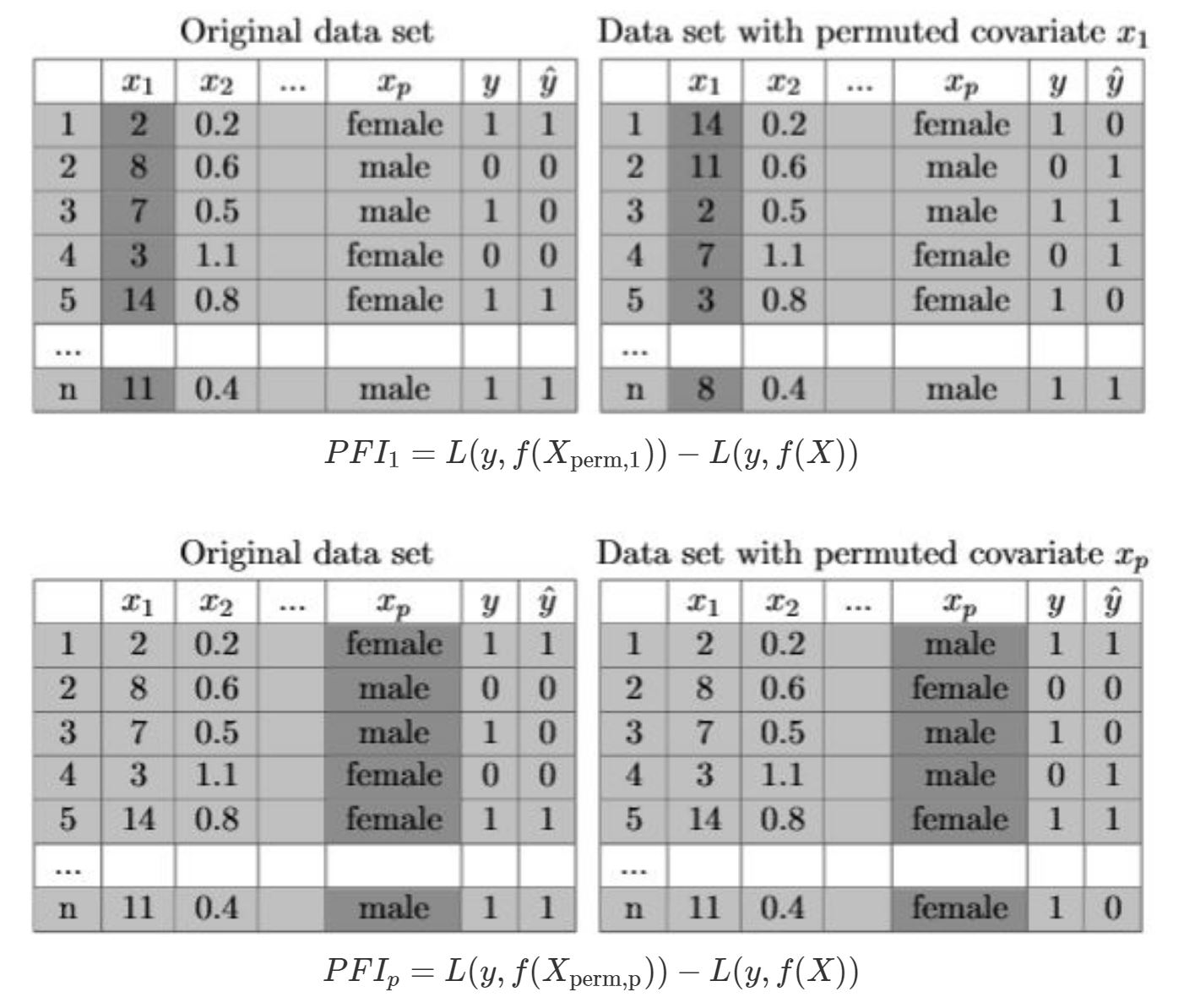
$Example for Permutation Feature Importance. The tables illustrate the second step of the algorithm of PFI, in particular the permutation of the features $x_{1}$ and $x_{p}$. As shown, the respective columns in dark grey are the ones which were shuffled. This breaks the association between the feature of interest and the target value. Based on the formula underneath the tables, the PFI is calculated.$

FIGURE 8.1: Example for Permutation Feature Importance. The tables illustrate the second step of the algorithm of PFI, in particular the permutation of the features $x_{1}$ and $x_{p}$. As shown, the respective columns in dark grey are the ones which were shuffled. This breaks the association between the feature of interest and the target value. Based on the formula underneath the tables, the PFI is calculated.

To show, how the PFI for all features of a model can be visualized and thereby more conveniently compared, the PFI algorithm with a random forest model is applied on the dataset "Boston" (see Figure 8.2), which is available in R via the MASS package. To predict the house price, seven variables are included, whereby as the results show, the PFI varies substantially across the variables. In this case, the features Status of Population and Rooms should be interpreted as the most important ones for the model, whereas Blacks is considered as less important.

Visualization of Permutation Feature Importance with a random forest applied on Boston dataset. The depicted points correspond to the median PFI over all shuffling iterations of one feature and the boundaries of the bands illustrate the 0.05- and 0.95-quantiles, respectively (see `iml` package).

FIGURE 8.2: Visualization of Permutation Feature Importance with a random forest applied on Boston dataset. The depicted points correspond to the median PFI over all shuffling iterations of one feature and the boundaries of the bands illustrate the 0.05- and 0.95-quantiles, respectively (see iml package).

8.2 Leave-One-Covariate-Out (LOCO)

The concept of Leave-One-Covariate-Out (LOCO) follows the same objective as PFI, to gain insights on the importance of a specific feature for the prediction performance of a model. Although applications of LOCO exist, where comparable to PFI, the initial values of feature $j$ are replaced by its mean, median or zero (see Hall, Phan, and Ambati 2017), and hence, circumvent the disadvantage of re-training the model $f$, the common approach follows the idea to simply leave the respective feature out. The overall prediction error of the re-trained model $f_{-j}$ is then compared to the prediction error resulted from the baseline model. However, re-training the model results in higher computational costs, which becomes more severe with an increasing feature space. Typically, one is interested in assessing the Feature Importance within a fixed model $f$. Applying LOCO might raise plausible concerns, as it compares the performance of a fixed model with the performance of a model $f_{-j}$ which is merely fitted with a subset of the data (see Molnar 2019). The pseudo-code shown below, illustrates the algorithm for the common case where the feature is left out (see Lei et al. 2018).

The Leave-One-Covariate-Out algorithm based on Lei et al. (2018):

Input: Trained model $f$, feature matrix $X$, target vector $y$, error measure $L(y,f(X))$

Estimate the original model error $e_{orig} = L(y,f(X))$ (e.g. mean squared error)
For each feature $j = 1,...,p$ do:
- Generate feature matrix $X_{-j}$ by removing feature j in the data $X$
- Refit model $f_{-j}$ with data $X_{-j}$
- Estimate error $e_{-j} = L(y,f_{-j}(X_{-j}))$ based on the predictions of the reduced data
- Calculate LOCO Feature Importance $FI_{j} = e_{-j}/e_{orig}$. Alternatively, the difference can be used: $FI_{j} = e_{-j} - e_{orig}$
Sort features by descending FI.

In Figure 8.3 it is shown, how the LOCO algorithm alters the original dataset, whereby it always differs, depending on the respective feature that is left out. Note, that the qualitative and quantitative interpretations correspond to the ones from the PFI method. So do the visualization tools and therefore at this point it is refrained from providing the reader with an additional real data example.

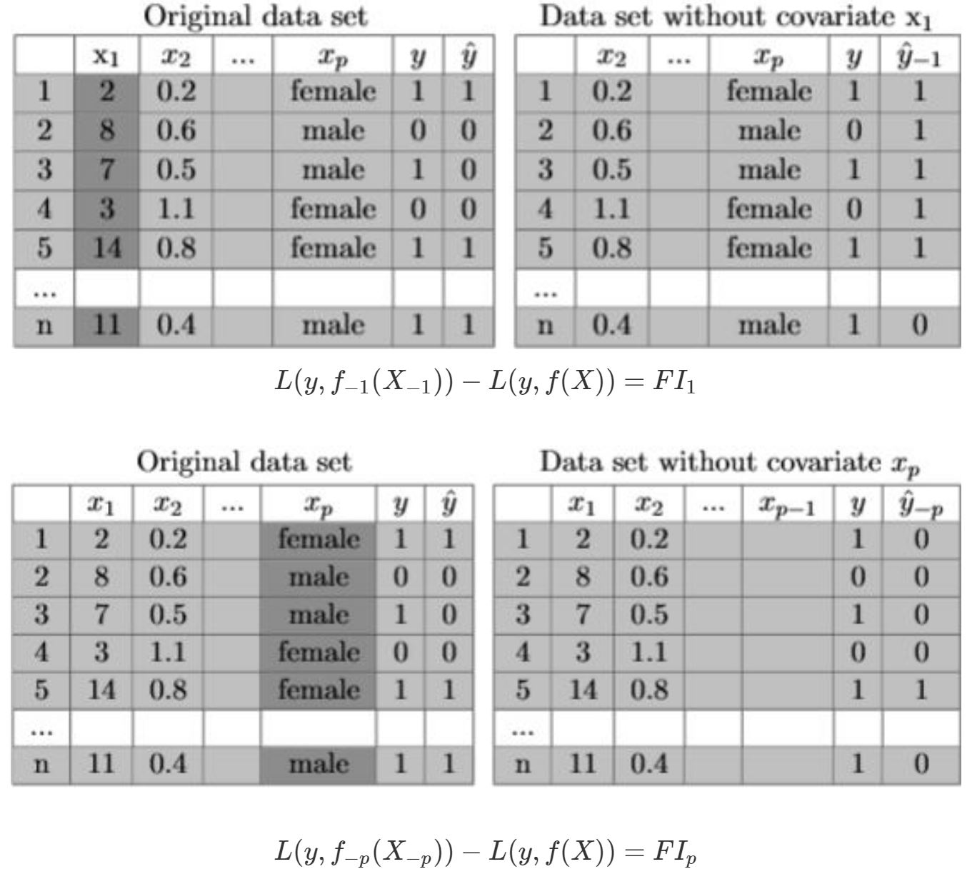
$Example for Leave-One-Covariate-Out Feature Importance. The tables illustrate the second step of the algorithm of LOCO in particular the drop of $x_{1}$ and $x_{p}$. The dark grey columns of the original dataset mark the variables that will be dropped and therefore ignored when refitting the model. This breaks the relationship between the feature of interest and the target value. Based on the formula underneath the tables, the Feature Importance of LOCO is calculated.$

FIGURE 8.3: Example for Leave-One-Covariate-Out Feature Importance. The tables illustrate the second step of the algorithm of LOCO in particular the drop of $x_{1}$ and $x_{p}$. The dark grey columns of the original dataset mark the variables that will be dropped and therefore ignored when refitting the model. This breaks the relationship between the feature of interest and the target value. Based on the formula underneath the tables, the Feature Importance of LOCO is calculated.

8.3 Interpretability of Feature Importance and its Limitations

After both methods are presented, it will be now questioned to what extent these agnostic-methods can contribute to a more comprehensive interpretability of machine learning models. Reflecting upon these limitations will constitute the main focus in the following chapters. Conveniently, both methods are highly adaptable on whether using classification or regression models, as they are non-rigid towards the prediction error metric (e.g. Accuracy, Precision, Recall, AUC, Average Log Loss, Mean Absolute Error, Mean Squared Error etc.). This allows to assess Feature Importance based on different performance measures. Besides, the interpretation can be conducted on a high-level, as both concepts do consider neither the shape of the relationship between the feature and outcome variable nor the direction of the feature effect. However, as illustrated in Figure 8.2, PFI and LOCO only return for each feature a single number and thereby neglect possible variations between subgroups in the data. Chapter 10 will focus on how this limitation can be, at least for PFI, circumvented and introduces the concepts of Partial Importance (PI) and Individual Conditional Importance (ICI) which both avail themselves on the conceptual ideas of PD and ICE (see Casalicchio, Molnar, and Bischl 2018). Besides, two general limitations appear when some features in the feature space are correlated. First, correlation makes an isolated analysis of the explanatory power of a feature complicated which results in an erroneous ranking in Feature Importance and hence, in incorrect conclusions. Second, if correlation exists and only in case of applying the PFI method, permuting a feature can result in unrealistic data instances so that the model performance is evaluated based on data which is never observed in reality. This makes comparisons of prediction errors complicated and therefore it should always be checked for this problem, if applying the PFI method. Chapter 9 will focus on this limitations by comparing the performance of PFI and LOCO for different models and different levels of correlation in the data. Beyond these limitations, it is evident to also question whether these agnostic-methods should be computed on training or test data. As answering that depends highly on the research question and data, it is refrained from going into more detail at this point but will be examined and further discussed in chapter 11.

References

Breiman, Leo. 2001a. “Random Forests.” Machine Learning 45 (1). Springer: 5–32.

Casalicchio, Giuseppe, Christoph Molnar, and Bernd Bischl. 2018. “Visualizing the Feature Importance for Black Box Models.” In Joint European Conference on Machine Learning and Knowledge Discovery in Databases, 655–70. Springer.

Fisher, Aaron, Cynthia Rudin, and Francesca Dominici. 2018. “Model Class Reliance: Variable Importance Measures for Any Machine Learning Model Class, from the” Rashomon” Perspective.” arXiv Preprint arXiv:1801.01489.

Hall, Patrick, Wen Phan, and Sri Satish Ambati. 2017. “Ideas on Interpreting Machine Learning.” O’Reilly Ideas.

Lei, Jing, Max G’Sell, Alessandro Rinaldo, Ryan J Tibshirani, and Larry Wasserman. 2018. “Distribution-Free Predictive Inference for Regression.” Journal of the American Statistical Association 113 (523). Taylor & Francis: 1094–1111.

Molnar, Christoph. 2019. Interpretable Machine Learning: A Guide for Making Black Box Models Explainable.