Chapter 13 LIME and Neighborhood
Author: Philipp Kopper
Supervisor: Christoph Molnar
This section will discuss the effect of the neighborhood on LIME's explanations. This is in particular critical for tabular data. Hence, we will limit ourselves to the analysis of tabular data for the remainder of this chapter.
As described in the previous chapter, LIME aims to create local surrogate models -- one for each observation to be explained. These local models operate in the proximity or neighborhood of the instance to be explained. They are fitted based on weights which indicate their proximity to the observation to be explained. The weights are typically determined using kernels that transform the proximity measure.
The proper parametrization of the kernel is obviously important. However, this is true for any approach that uses kernels, such as kernel density estimations. Figure 13.1 illustrates kernel densities from a standard normal distribution. We applied different kernel widths for the curve estimation.
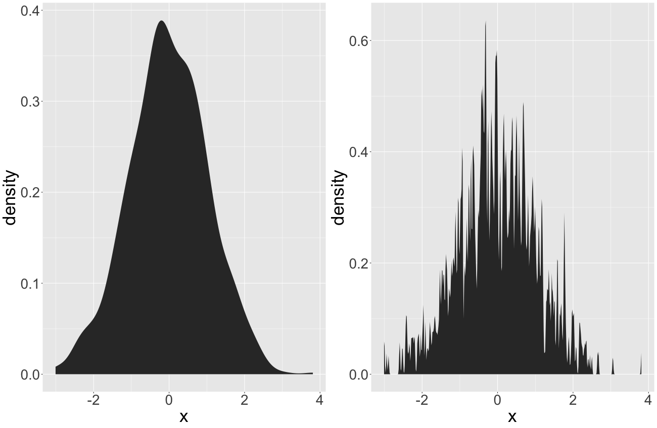
FIGURE 13.1: In(appropriate) kernel widths for kernel density estimations. The left panel illustrates an appropriate kernel width. The right one features an inappropriate one.
One can easily see that the left panel seems to be appropriate while the right one is too granular. The proper definition of the neighborhood is very crucial in this case. However, with no prior information, this definition is arbitrary.1 We can only judge on the proper definition of the neighborhood from our experience and our expectations. This may work in low dimensional problems and descriptive statistics. However, machine learning models operate in multivariate space and mostly tackle complex associations. Thus, it seems much harder to argue on the proper neighborhood definition when working with LIME.
This chapter reviews the neighborhood issue of the LIME algorithm critically. The objective of this chapter is rather to outline this particular issue and not to suggest solutions for it. First of all, it describes the neighborhood definition abstractly in greater detail (section 13.1). Then, it illustrates how problematic the neighborhood definition can be in a simple one-dimensional example in section 13.2. Furthermore, we study the effect of altering the kernel size more systematically in more complex contexts in the next section (13.3). This section deals with both, simulated (13.3.1) and real (13.3.2) data. The first subsection of the simulation (13.3.1.1) investigates multivariate globally linear relationships. The second one (13.3.1.2) researches local coefficients. The third one (13.3.1.3) studies non-linear effects. Section 13.3.2 uses the Washington D.C. bicycle data set to study LIME's neighborhood in a real-world application. Afterwards, in section 13.4, we discuss the results and contextualize them with the existing literature. After concluding, we explain how LIME was used and why in section 13.5.
13.1 The Neighborhood in LIME in more detail
When obtaining explanations with LIME, the neighborhood of an observation is determined when fitting the model by applying weights to the data. These weights are chosen w.r.t. the proximity to the observation to be explained. However, there is no natural law stating that local models have to be found this way. Alternatively, Craven and Shavlik (1996) show that increasing the density of observations around the instance of interest is very helpful to achieve locally fidele models. Hence, locality could be obtained in many more different ways than weighting observations combined with global sampling as it is in LIME. After sampling, the data points are weighted w.r.t. their proximity to the observation to be explained. One possible alternative to this procedure might be to combine steps 2 (sampling) and 4 (weighting) of the LIME algorithm2 to a local sampling. This way we would increase the density around the instance already by proper sampling. In fact, Laugel et al. (2018) claim that this way should be preferred over the way LIME samples. In this chapter, however, we focus on the explicit implementation of LIME and analyze how the weighting strategy ceteris paribus affects surrogate model accuracy and stability.
When working with LIME, the weighting of instances is performed using a kernel function over the distances of all other observations to the observation of interest. This leaves us arbitrary (in fact, they may not be that arbitrary) choices on two parameters: the distance and the kernel function. Typical distance functions applicable to statistical data analysis are based on the L0, L1 and L2 norms. For numerical features, one tends to use either Manhattan distance (L1) or Euclidean distance (L2). For categorical features, one would classically apply Hamming distance (L0). For mixed data (data with both categorical and numerical features), one usually combines distances for numerical and categorical features. So does Gower's distance (Gower (1971)) or the distance proposed by Huang (1998):
\[ d_H(x_i, x_j) = d_{euc}(x_i, x_j) + \lambda d_{ham}(x_i, x_j) \]
with \(d_{euc}\) referring to the Euclidean distance and \(d_{ham}\) to the Hamming distance. \(d_{euc}\) is only computed for numerical and \(d_{ham}\) only for categorical ones. \(\lambda\) steers the importance of categorical features relative to numerical ones. Huang (1998) recommends setting \(\lambda\) equal to the average standard deviation of the numerical features. For scaled numerical features (standard deviation is one) this metric is equivalent to the Euclidean distance. It is important to note that despite these existing measures it may be challenging to properly determine distances for mixed data. For text data, M. T. Ribeiro, Singh, and Guestrin (2016b) recommend using cosine distance and Euclidean distance for images.
For the kernel function itself, there are two parameters to be set. First of all, the type of kernel. Second, the kernel width. By default, the R implementation uses an exponential kernel where the kernel width equals the square root of the number of features.
The choice of the distance measure seems least arbitrary. Furthermore, the choice of the kernel function is not expected to have the most crucial impact on the neighborhood definition. Thus, we focus on the kernel width in our experimental study.
13.2 The problem in a one-dimensional setting
How crucial the proper setting of the kernel width can be, is illustrated by a very simple example. We simulate data with one target and two features. One feature is pure noise and the other one has a non-linear sinus-like effect on the target. If we plot the influential feature on the x-axis and the target on the y-axis, we can observe this pattern in figure 13.2.
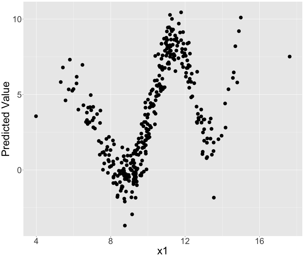
FIGURE 13.2: Simulated data: The non-linear relationship between the feature and the target.
Now we fit a random forest on this data situation which should be able to detect the non-linearity and incorporate it into its predictive surface. We observe that the predictions of the random forest look very accurate in figure 13.3. Only on the edges of the covariate (where the density is lower) the random forest turns out to extrapolate not optimally.
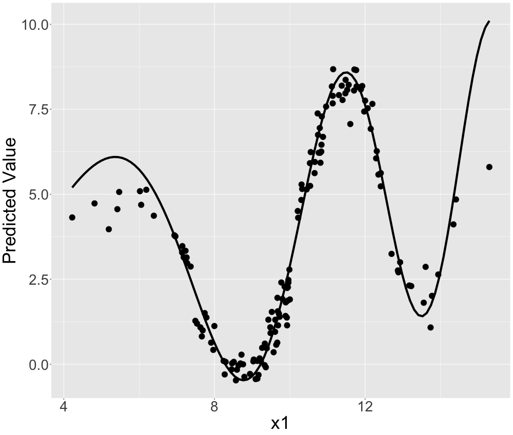
FIGURE 13.3: Simulated data: Random forest predictions for non-linear univariate relationship. The solid line represents the true predictive surface.
LIME could now be used to explain this random forest locally. "Good" local models would look very different w.r.t. the value of the feature, x1. For example, we could describe the predictions locally well by piece-wise linear models. This is depicted in figure 13.4.
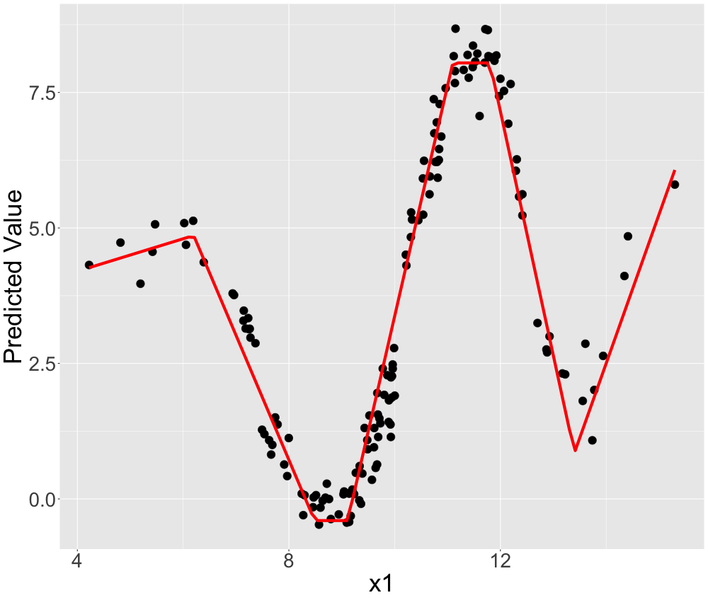
FIGURE 13.4: Simulated data: Non-linear univariate relationship explained by a piece-wise linear model.
LIME should be able to find these good local explanations -- given the right kernel size. Let's select one instance which we want an explanation for. We illustrate this instance by the green point in figure 13.5. This particular instance can be approximately linearly described by a linear regression with intercept \(60\) and slope \(-4.5\). If we set the kernel width to \(0.08\), we fit this local model. This is indicated by the red line in figure 13.5. However, if we increased the kernel width to \(2\), the coefficients change to \(-2.84\) (intercept) and \(0.64\) (slope) (on average) which seems drastically distorted as observed by the yellow line in figure 13.5. The yellow line does not seem to fit a local linear model but rather a global one.
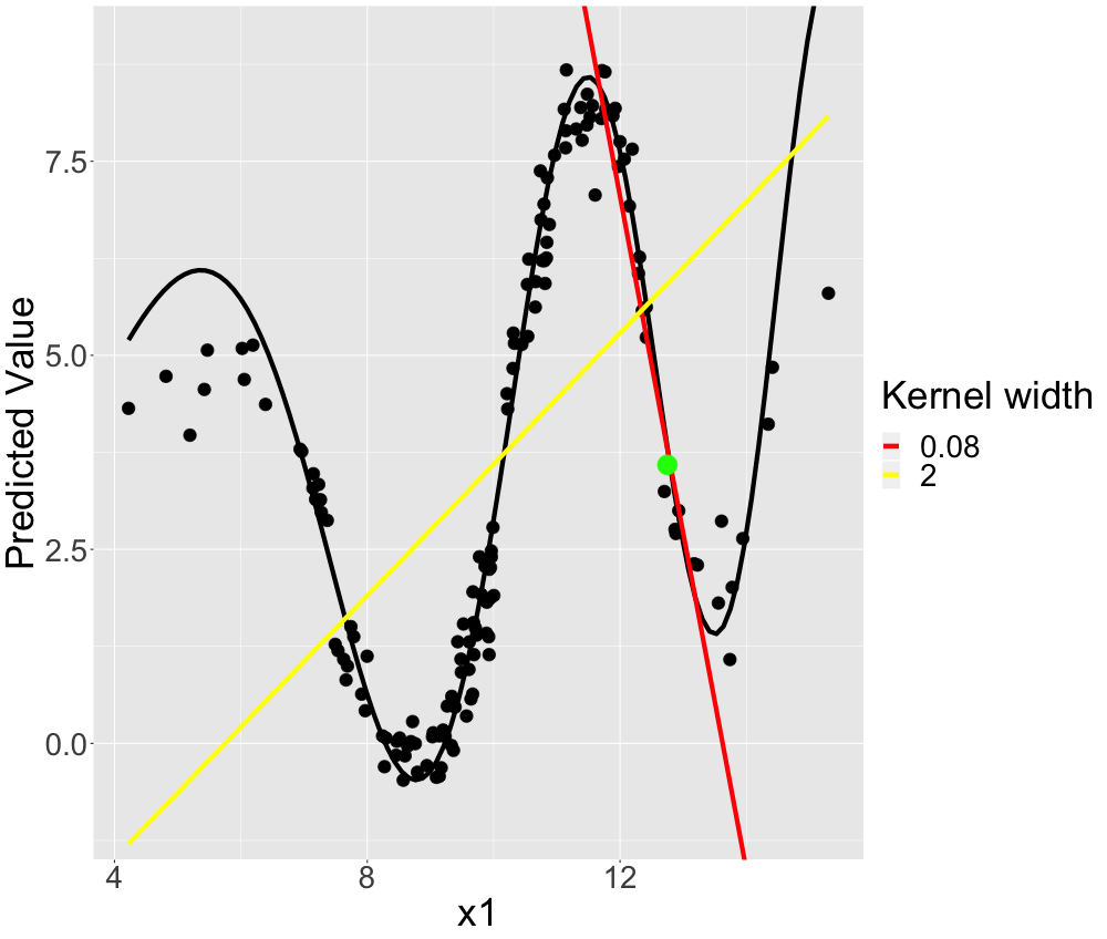
FIGURE 13.5: Simulated data: Possible local (LIME) models for the non-linear univariate relationship.
As a next step, we review explanations resulting from altering the kernel size in figure 13.6 more systematically. We average over many different models to achieve more robust local models. We do that because we observe some coefficient variations resulting from the (random) sampling in the LIME algorithm. In figure 13.6 (upper panel) we see these averaged models for different kernel sizes. We observe that the larger we set the kernel size, the more we converge to a linear model that operates globally. The largest three kernel sizes (\(0.5\), \(1\) and \(2\)) appear very global while \(0.05\) and \(0.1\) seem to fit good local models. \(0.25\) and \(0.3\) are neither global nor very local. This is very intuitive and complies with the idea of a weighted local regression.
Additionally, we analyze the same alteration of the kernel size for an observation where a good local approximation would be a linear model with a positive slope in the lower panel of figure 13.6. We observe a similar behavior.
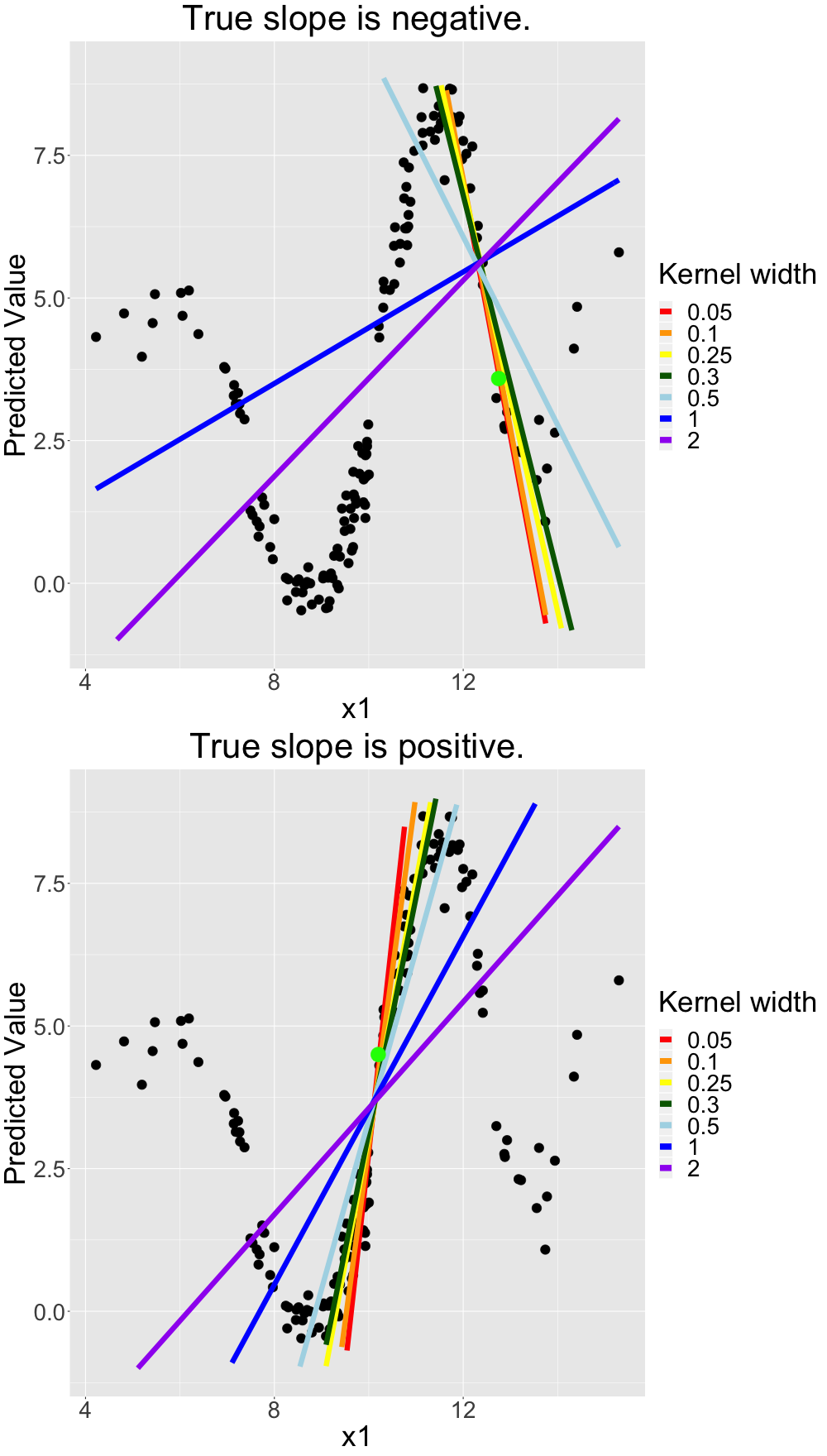
FIGURE 13.6: Simulated data: Local (LIME) models for non-linear univariate relationship with different kernel sizes for different observations.
This behavior is not necessarily a problem but only a property of LIME. However, it can be problematic that the appropriate kernel size is not a priori clear. Additionally, there is no straight forward way to determine a good kernel width for a given observation to be explained. The only generic goodness-of-fit criterion of LIME, model fidelity, is not necessarily representative: If we set the kernel size extremely small there will be many models with an extremely good local fit as local refers only to a single observation. In our examples, it looks as if a very small kernel size should be preferred. A small kernel width indeed grants local fit. But what a small kernel width means, also strongly depends on the dimensionality and complexity of the problem.
13.3 The problem in more complex settings
The previous setting was trivial for LIME. The problem was univariate and we could visualize the predictive surface in the first place. This means that interpretability was mostly given. We will study our problem in more complex -- non-trivial -- settings to show that it persists. We will do so by examining simulated and real data.
13.3.1 Simulated data
We simulate data with multiple numeric features and a numeric target. We assume the features to originate from a multivariate normal distribution where all features are moderately correlated. We simulate three different data sets. In the first one, the true associations are linear (globally linear). In the second one, the true associations are linear but only affect the target within a subinterval of the feature domain (locally linear).3 In the third one, we simulate globally non-linear associations. For all three data sets, we expect the kernel width to have an impact on the resulting explainer. However, for the global linear relationships, we expect the weakest dependency because the true local model and the true global model are identical. Details on the simulation can be obtained in our R code and section 13.3.1.1.
13.3.1.1 Global Linear Relationships
We simulate data where the true predictive surface is a hyperplane. Good machine learning models should be able to approximate this hyperplane. This case is -- again -- somewhat trivial for LIME. The most suitable model for this data would be linear regression which is interpretable in the first place. Thus, LIME can be easily tested in this controlled environment. We know the true local coefficients as they are equal to the global ones. We can evaluate the suitability of the kernel width appropriately.
The simulated data looks as follows: The feature space consists of three features (\(x_1\), \(x_2\), \(x_3\)). All originate from a multivariate Gaussian distribution with mean \(\mu\) and covariance \(\Sigma\). \(\mu\) is set to be \(5\) for all features and \(\Sigma\) incorporates moderate correlation. The true relationship of the features on the target \(y\) is described by:
\[ y = \beta_0 + \beta_1 x_1 + \beta_2 x_2 + \beta_3 x_3 + \epsilon \] We set the true coefficients to be \(\beta_1 = 4\), \(\beta_2 = -3\), \(\beta_3 = 5\).
We use linear regression (the true model) as a black box model. Using cross-validation, we confirm that the model has a high predictive capacity -- approaching the Bayes error. Not surprisingly, the linear model describes the association very well.
We choose random observations and compute the local LIME model for each one of them w.r.t. different kernel sizes. We expect that the kernel size may be infinitely large as the global model should equal good local models. However, if the kernel width is set too small we may fit too much noise. Hence, in this case, we may find no good local models.
The figures below (all four panels of figure 13.7) indicate the local parameters for one of the selected observations for different kernel sizes which have been determined by LIME. The three vertical lines indicate the true global coefficients. This behavior is representative of all observations.
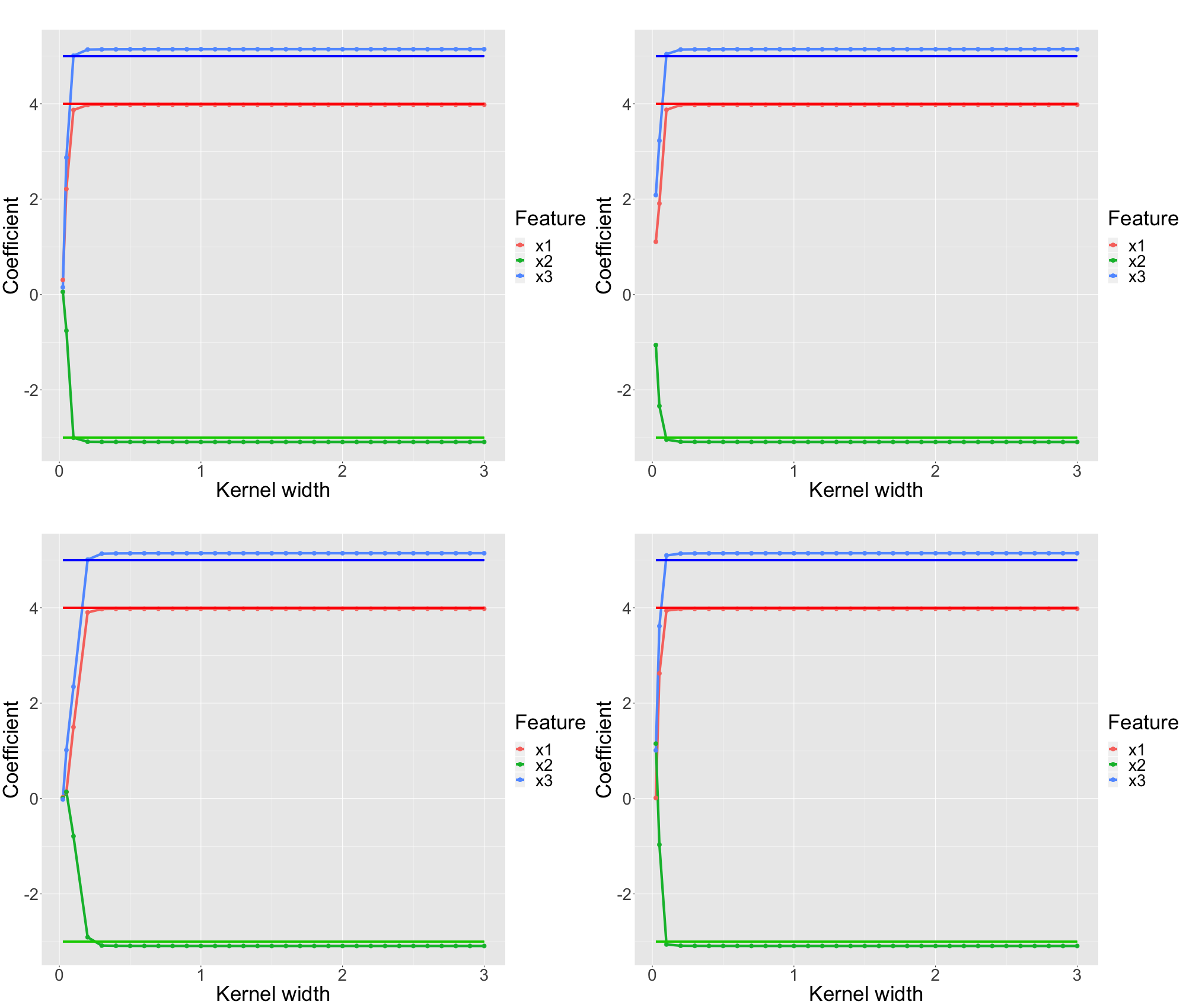
FIGURE 13.7: Simulated data: Each panel represents a single (representative) observation. For each observation we analyze the LIME coefficients for different kernel widths. The underlying ground truth model is a linear model. Each feature is depicted in a different color. The solid vertical lines represent the true coefficient of the LIME explanation.
We observe that too small kernel widths are not able to reproduce the global predictive surface at all. However, provided the kernel width is not too small, all kinds of kernel widths from small size to very large kernels fit very similar models which are all very close to the true model.
These results allow concluding that for explaining linear models the kernel width is a non-critical parameter. However, this case may be seen as trivial and tautological for most users of LIME. Still, this result is valuable as it shows that LIME works as expected.
13.3.1.2 Local Linear Relationships
For non-linear relationships, we have already seen that the kernel width is more crucial. Thus, we aim to study the behavior of the explanations w.r.t. the kernel size where the true associations are non-linear or locally different.
We may induce non-linearity by different means. However, first of all it seems interesting to study how the kernel width affects LIME explanations in a very simple form of non-linearity: The features only affect the target locally linearly, as expressed by:
\[ y = \beta_0 + \beta_1 x_1 1_{x_1<c_1} + \beta_2 x_2 + \beta_3 x_3 + \epsilon + \gamma_0 1_{x_1>c_1} + \epsilon_i\]
where \(x_1\) only affects \(y\) within the given interval. \(\gamma_0\) corrects the predictive surface by another intercept to avoid discontinuities. This time, we fit a MARS (multivariate adaptive regression splines) model (Friedman and others (1991)) which can deal with this property of local features. In theory, MARS can reproduce the data generating process perfectly and hence is our first choice. Using cross-validation we confirm that the model has a high predictive capacity. However, note that all of our results would be qualitatively (MARS turns out to feature clearer results.) identical between MARS and random forest. Given an appropriate kernel, LIME should succeed in recovering the local predictive surface.
We set \(\beta_1 = 5\), \(\beta_2 = -4\), \(\beta_3 = 3\) and \(c_1 = 5\). This means that the slope of \(\beta_1\) equals to \(5\) until \(x_1 = 5\) and to \(0\) afterwards. This results in an average slope of \(2.5\) over the whole domain.
We investigate representative observations, i.e. belonging to each bin of the predictive surface to check if LIME recovers all local coefficients.
Hence, representative means that we should investigate observations with the following properties:
\(x_1 < 5\)
\(x_1 > 5\)
We think these observations are best explained in areas with reasonable margin to \(x_1 = 5\).
Below in figure 13.8, we depict the coefficient paths for four representative observations, two belonging to each bin (upper panels: \(x_1 < 5\), lower panels: \(x_1 > 5\)). The true local coefficients are displayed by solid vertical lines.
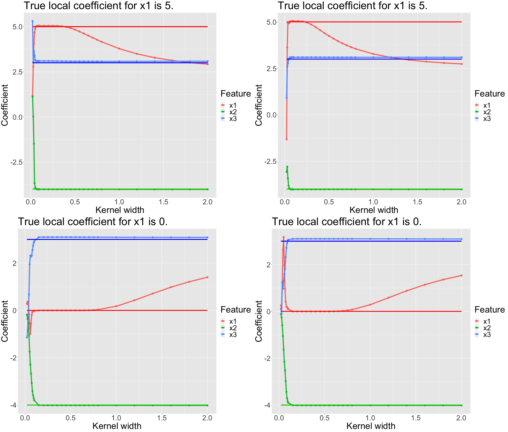
FIGURE 13.8: Simulated data: Each panel represents a single (representative) observation. For each observation we analyze the LIME coefficients for different kernel widthss. The underlying ground truth model is a linear model where x1 only has a local coefficient. Each feature is depicted in a different color. The solid vertical lines represent the true coefficient of the LIME explanation.
We can see that in this case, we cannot simply set an arbitrary kernel width. The true local coefficient for \(x_1\) is only approximated well within a limited interval of the kernel width. In our scenario, good kernel widths are between \(0.1\) and \(0.7\) (while the upper bound varies for the observations). As before, we observe that a too-small kernel width (\(< 0.1\)) produces non-meaningful coefficients. On the other hand, for large kernel widths (\(> 0.7\)) the true coefficient is not approximated, but rather the global (average) linear coefficient: For \(x_1\) a large kernel width results in a linear model that averages the local slopes. More formally, one could describe this sort of explanation as a global surrogate model. Additionally, we observe that for smaller kernel widths, the local models are rather volatile. More systematically, Alvarez-Melis and Jaakkola (2018) investigate this volatility and find that LIME is prone to finding unstable explanations.
This motivates us to further research the volatility. We display the mean and the confidence intervals of the coefficients of 100 different models for different kernel sizes in figure 13.9 for \(x_1\). The black lines interpolate averaged coefficient estimates for different kernel sizes. The solid black line indicates the true local coefficient. The grey shaded area represents the (capped) 95% confidence intervals. For very low kernel widths we observe massive volatility. The volatility decreases to an acceptable level only after \(0.1\) for all covariates.
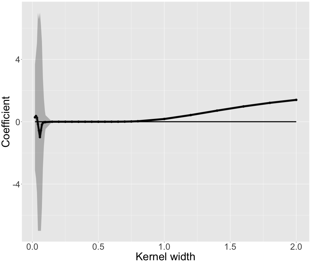
FIGURE 13.9: Simulated data: For one observation we display the local coefficient and confidence intervals for different kernel widths. The underlying ground truth model is a linear model where x1 only has a local coefficient. Hence, we only investigate x1.
Note that we obtain the same picture for every covariate and other representative observations. We observe that there is a trade-off between stable coefficients and locality (expressed by a small kernel width). Our analysis suggests the following: Too large kernel sizes result in explanations biased towards a global surrogate. At the same time, the kernel width must result in stable coefficients. This means we cannot set it infinitesimally small. The resulting trade-off suggests choosing the minimal kernel size with stable coefficients as an optimal solution. Mathematically speaking, we aim minimal kernel size which still satisfies a volatility condition.
13.3.1.3 Global Non-Linearity
We further generalize the approach from the previous section and simulate data with the underlying data generating mechanism:
\[ y = \beta_0 + \beta_1 x_1 + \beta_{2,1} x_2 1_{x_2<c_1} + \beta_{2,2} x_2 1_{c_1 < x_2 < c_2} + \beta_{2,3} x_2 1_{c_2 < x_2} + \beta_3 x_3 + \epsilon \]
where the slope \(\beta_2\) is piece-wise linear and changes over the whole domain of \(x_2\). We set \(\beta_1 = 5\), \(\beta_{2,1} = -4\), \(\beta_{2,2} = 3\), \(\beta_{2,3} = -3\) \(\beta_3 = 3\), \(c_1 = 4\) and \(c_2 = 6\).
We omitted the support intercepts \(\gamma_0 1_{c_1 < x_1 < c_2} + \gamma_0 1_{x_1 > c_2}\) in the equation above (which guarantee continuity).
We study three representative observations complying with:
\(x_2 < 4\)
\(4 < x_2 < 6\)
\(6 < x_2\)
As before, we use a MARS model as our black box. When explaining the black box with LIME, we observe the same pattern as before. Figures 13.10 and 13.11 look very similar to the corresponding figures of the previous section. However, the intervals of "good" solutions are -- naturally -- much smaller. The more complex the true associations become, the more we observe this trend of decreasing solution intervals. It seems as if the more complex the predictive surface is, the harder it is for LIME to even find a good local model.
For globally non-linear associations, we also find that we prefer a small kernel which however also produces stable coefficients.
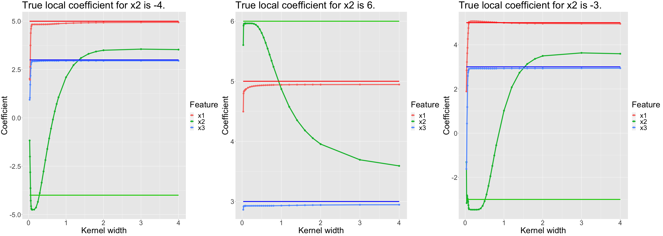
FIGURE 13.10: Simulated data: Local coefficients for different kernel widths explaining non-linear relationship (for \(x_2\)).
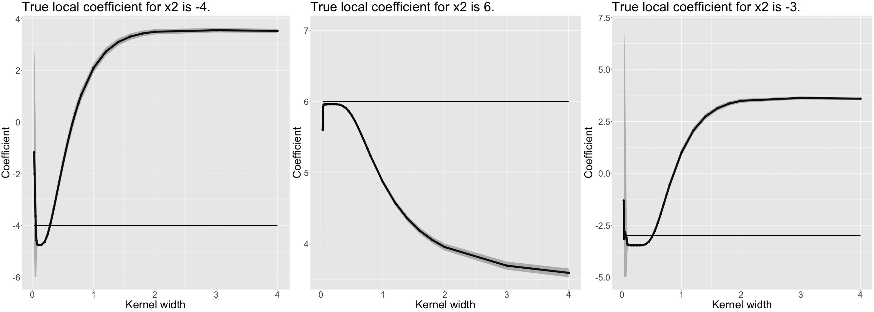
FIGURE 13.11: Simulated data: Local coefficients and confidence intervals for different kernel widths explaining non-linear relationship (for \(x_2\)).
Having investigated simulated data where we knew the ground truth, gave us a good intuition on how the kernel size affects the resulting explainer model. The neighborhood problem can be described briefly by the following. A (too) small kernel width usually worsens coefficient stability whilst a too large kernel width fits a global surrogate model. An optimal kernel size should balance these effects. We may formulate the problem as a minimization problem w.r.t. the kernel size. However, the minimization needs to consider the constraint that coefficients need to be stable.
13.3.2 Real data
Leaving the controlled environment may make things more difficult. Relevant challenges include:
High-dimensional data may be an issue for the computation of the kernel width. LIME computes dissimilarities. It is well-known that (some) dissimilarities get increasingly less meaningful as the feature space expands. This is one consequence of the curse of dimensionality.
Computing some dissimilarities (e.g. Manhattan or Euclidean) also comes with the problem that the cardinality of the features mainly steers this measure. Thus, LIME should always apply scaling.
When working with real data sets with many features, we typically want a sparse explanation. To achieve this, we should let LIME perform feature selection.
Luckily, the latter two are featured in the Python and R implementations.
Within this section, we study whether we can confirm our simulated data findings for real-world data. We will work with the well-known Washington D.C. bicycle rental data set. This dataset contains daily bicycle hire counts of a Washington D.C. based rental company. The data has been made openly available by the company itself (Capital-Bikeshare). Fanaee-T and Gama (2014) added supplementary information on the weather data and season associated with each day. For details on the data set please refer to Molnar (2019) (https://christophm.github.io/interpretable-ml-book/bike-data.html). We select this data set because it is well-known in the machine learning community and this regression problem is easily accessible to most people. Furthermore, it has a reasonable feature space making it not highly prone to the curse of dimensionality of the distance measures. We only make use of a subset of all possible features as some are somewhat collinear.
Using this data we aim to use a random forest to predict the number of daily bicycle hires. We use LIME to explain the black box.
When working with LIME in practice, we want to obtain stable explanations. An explanation is stable if the surrogate model does not change much when altering the randomly drawn samples. We evaluate this property with the aid of a modified version of stability paths (Meinshausen and Bühlmann (2010)). Stability paths are used for sparse (regularised) models and indicate how likely each covariate is part of the model -- w.r.t. a given degree of regularisation. Normally, they analyze the association of the regularisation strength and inclusion probabilities of features. On the x-axis, one depicts the regularisation strength and on the y-axis the inclusion probabilities (for all covariates). The probabilities for different regularisations are grouped by feature.
However, for LIME we rather aim to study how likely a covariate is part of the (sparse) model over a grid of kernel widths. Our motivation to use stability paths is that they are easier to interpret compared to coefficients paths (or similar evaluation methods) in our setting.
Over a grid of kernel widths (from almost 0 to 20), we compute multiple sparse explanations for the same kernel width. Sparse means that we limit our explainer to only the three most influential local features. We count how frequently each covariate has been part of the explanation model (out of all iterations). We divide by the total number of iterations and achieve estimates for the sampling probability for a given observation, a given number of features and a given kernel width. We search the full (predefined) grid of kernel widths. We can repeat this procedure for any other observation.
Our pseudo stability paths are stable in areas where we have extreme probabilities, i.e. either probabilities close to 1 or close to 0. Furthermore, they should not change extremely when the kernel width slightly changes.
Figure 13.12 displays ideal stability paths with the three distinct areas observed earlier:
High variability for small kernels.
Local stability for optimal kernels.
Convergence to a global surrogate for large kernels.
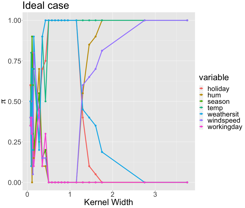
FIGURE 13.12: Real data: Example for ideal stability paths with three distinct areas. The x-axis displays different kernel widths. The y-axis indicates the respective inclusion probability of each variable. The variables are grouped by color.
The (toy example) stability paths suggest that temperature, weather situation and holiday are the local features while temperature, humidity and wind speed are deemed as the global ones.
This figure would help us to clearly identify a stable local model. However, in real life, things mostly are more complex. In figure 13.13, we display the stability paths for different selected observations for our random forest.
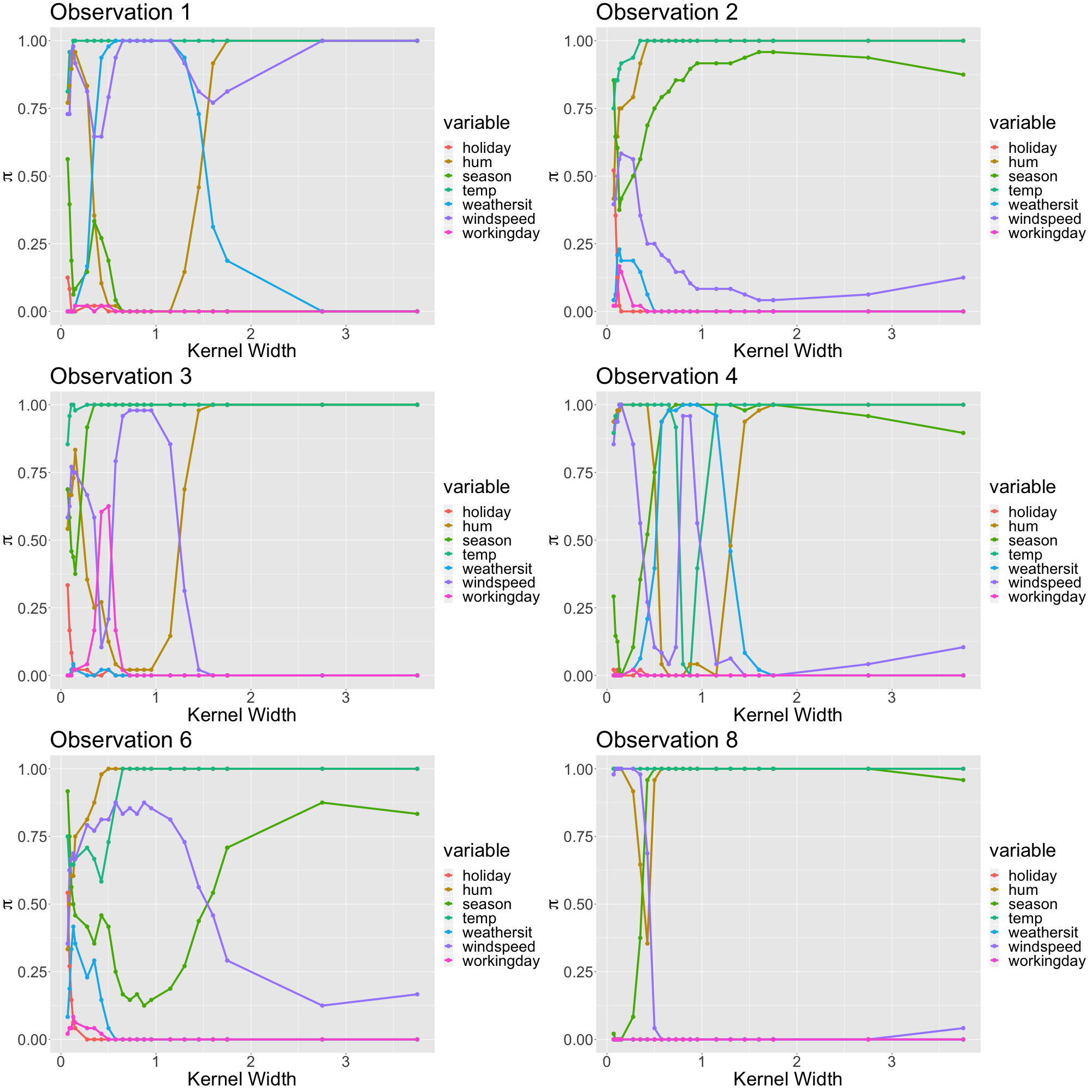
FIGURE 13.13: Real data: Stability paths for different observations from the bycicle data set explaining a random forest.
We observe that stability paths converge to a set of covariates if we set the kernel width large. These are the global features. There is one interesting observation about this. Different observations sometimes converge to different global surrogate models. The covariates humidity and temperature are always selected. Then, either the windspeed (e.g. only observation 1) or the season (the remainder observations) is selected as global feature. We believe that this is because both covariates are similarly strong on the global scope. Globally evaluating the feature importance of the random forest suggests that in fact temperature, season, humidity and wind speed are the most relevant features.
Furthermore, we observe that for small values of the kernel width, we have -- like in our simulation -- high variation. Here, this variation is expressed by intersecting paths where most covariates are (almost) equally likely to be sampled.
For some observations, there seems to be a narrow range where there are stable and local explanations. For instance, consider observations 1 and 3. Here, the local models seem quite clear. For observation 1, between kernel widths of \(0.5\) and \(1\) it seems as if the temperature, the wind speed, and the weather situation are most influential. For observation 3, the selected local features are temperature, wind speed and season. For other observations, such as observations 4 and 8, we may argue that there are local and stable explanations, too. These are, however, by far less convincing than the previous ones. Additionally, we are struggling to identify stable local models for many observations, like observation 2 and 6. For those observations, there is only instability for small kernel widths which transforms immediately to the global surrogate once stabilized. The reasons for this variation of behavior can be manifold. However, not knowing the ground truth, it is hard to evaluate what is going on here in particular.
So even though we may find meaningful explanations from case to case, there is too much clutter to be finally sure about the explanations' goodness. Furthermore, "local" explanations still seem quite global as they seem quite similar for many different observations. Considering our explanations, the sparse models were highly correlated consisting of similar features for different observations. The only truly stable explanations remain essentially global ones with large kernel width. It seems as if the predictive surface is too complex to facilitate local and stable surrogate models properly. The curse of dimensionality affects locality very strongly. As distances in higher-dimensional Euclidean space are increasingly less meaningful, the definition of locality is very poor with an increasing number of features.
Summarizing, we observe both effects being described in the literature also for our real data example: instability (Alvarez-Melis and Jaakkola (2018)) for small kernel widths and global surrogates (Laugel et al. (2018)) for large ones. For simulated data, we can observe these effects as well. At the same time, we can identify local and stable explanations in this controlled environment. For real data, however, it is hard to locate the area which we identified for simulated data where we find a stable and local model.
13.4 Discussion and outlook
LIME is capable of finding local models. We show this using simulated data. The specification of a proper kernel width is crucial to achieving this. A proper locality is expressed by the minimal kernel width producing stable coefficients. However, we see that it is difficult to find these models in practice. We are unable to detect explanations that were both, stable and local, for our real data application -- at least with certainty. We largely observe the pattern described by Laugel et al. (2018) who claim that LIME explanations are strongly biased towards global features. At the same time, our study agrees with Alvarez-Melis and Jaakkola (2018) who find that local explanations are highly unstable. We confirm these findings using the bicycle rental data set. Additionally, also for simulated data, it becomes harder to detect a good locality if the predictive surface becomes more complex.
Similar results can be obtained for alternative data sets. For the practitioner using LIME (for tabular data), this means that LIME should be used with great care. Furthermore, we suggest analyzing the resulting explanations' stability when making use of LIME.
We think that the global sampling of LIME is responsible for many of the pitfalls identified. Hence, we propose that LIME should be altered in the way proposed by Laugel et al. (2018) to LIME-K. Local sampling should replace global sampling to better control for the locality.
Even though having said this, we think that LIME is one of the most promising recent contributions to the Interpretable Machine Learning community. The problems described in this chapter are mainly associated with tabular data. Domains where LIME has been applied successfully include image data and text data. Within these domains, LIME works differently from tabular data. For example, LIME's sampling for text data is already very local. It only creates perturbations based on the instance to be explained.
13.5 Note to the reader
13.5.1 Packages used
For our analysis, we used R (R Core Team (2020)). For all black box models, we used the mlr package (Bischl et al. (2020)) and the lime package (Pedersen and Benesty (2019)) for the LIME explanations. All plots have been created using ggplot2 (Wickham et al. (2020)).
13.5.2 How we used the lime R package and why
Using the lime package we heavily deviated from the default package options. We strongly recommend to not bin numerical features. The next chapter will outline in detail why this is not a good idea. In the first place, the main argument for binning has been enhanced interpretability. We suggest, though, that the same interpretability can be obtained by the absolute contribution of the feature to the prediction. This means, instead of the local coefficient, LIME should rather print the local coefficient times the feature value within its explanation. This argument makes binning -- provided that there is no additional benefit except interpretability (Refer to the next chapter.) -- obsolete.
While we think Gower distance is an interesting approach to deal with mixed data, we explicitly promote not to use it. In the current (July 2019) R implementation, when working with Gower distance there is no kernel applied. Explanations do not correspond to altering the kernel width. As we have seen, a proper kernel width may look very different depending on the associated problem. So it is highly unlikely that a one-size-fits-all implicit kernel width always results in a proper result. In figure 13.14 we analyze this statement by comparing the Gower distance's local coefficient to the true coefficient and the local estimates of the non-linear data simulation from section 13.3.1.3.
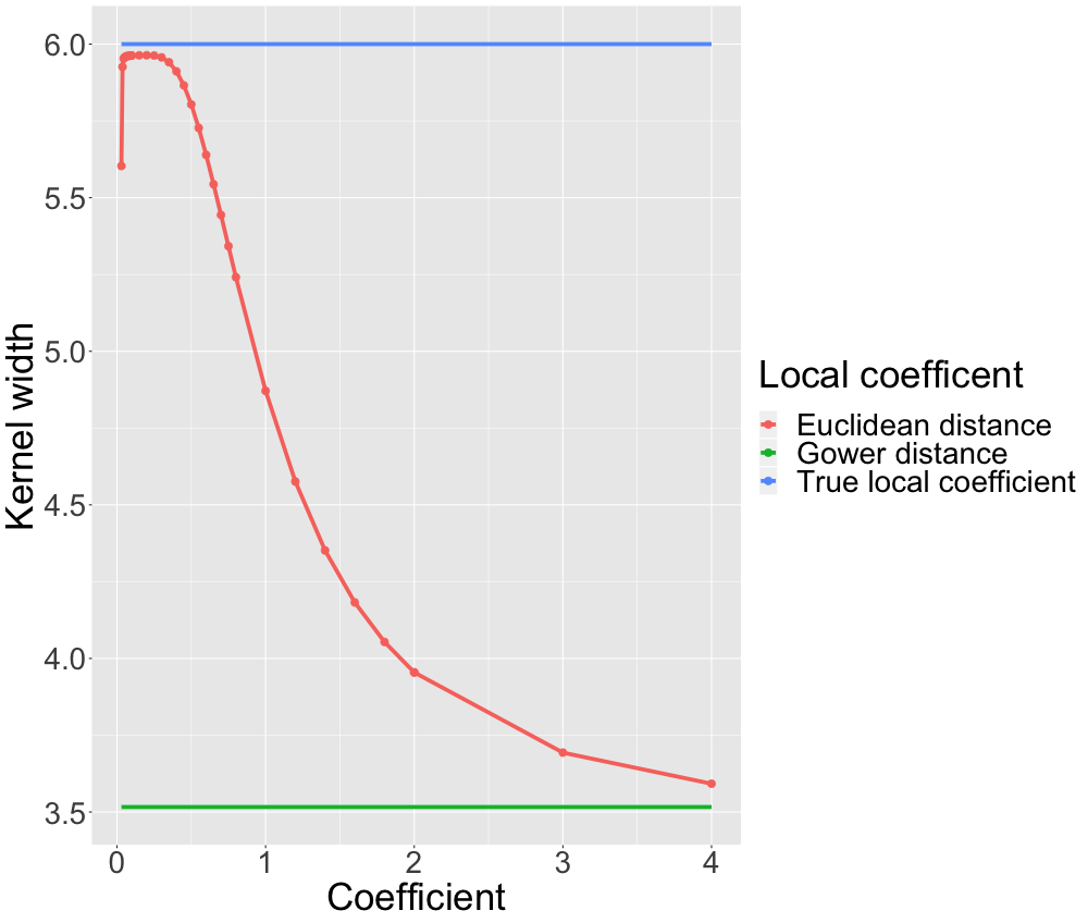
FIGURE 13.14: Simulated data: Gower distance vs. Euclidean distance (non-linear relationship). The blue line is the true coefficient. The interpolated curve represents the LIME coefficient estimates for different kernel widths when using Euclidean distance. The green line represents to estimate resulting from LIME when using Gower distance.
We see that our argument is valid. Gower distance is not able to recover the true coefficients and acts as a global surrogate.
Even though we think that Gower distance may result in some cases in good local models, its (currently) lacking flexibility most likely causes either instable or global explanations.
Usually, LASSO is the preferred option for variable selection as it is less seed dependent than, let's say, step-wise forward selection. However, we do not use LASSO but step-wise forward selection because the current implementation of LASSO has shortcomings and does not deliver results suitable for our analysis.
All in all, we strongly discourage the user of the lime R package to use the default settings.
References
Alvarez-Melis, David, and Tommi S Jaakkola. 2018. “On the Robustness of Interpretability Methods.” arXiv Preprint arXiv:1806.08049.
Bischl, Bernd, Michel Lang, Lars Kotthoff, Patrick Schratz, Julia Schiffner, Jakob Richter, Zachary Jones, Giuseppe Casalicchio, and Mason Gallo. 2020. Mlr: Machine Learning in R. https://CRAN.R-project.org/package=mlr.
Craven, Mark, and Jude W Shavlik. 1996. “Extracting Tree-Structured Representations of Trained Networks.” In Advances in Neural Information Processing Systems, 24–30.
Fanaee-T, Hadi, and Joao Gama. 2014. “Event Labeling Combining Ensemble Detectors and Background Knowledge.” Progress in Artificial Intelligence 2 (2-3). Springer: 113–27.
Friedman, Jerome H, and others. 1991. “Multivariate Adaptive Regression Splines.” The Annals of Statistics 19 (1). Institute of Mathematical Statistics: 1–67.
Gower, John C. 1971. “A General Coefficient of Similarity and Some of Its Properties.” Biometrics. JSTOR, 857–71.
Huang, Zhexue. 1998. “Extensions to the K-Means Algorithm for Clustering Large Data Sets with Categorical Values.” Data Mining and Knowledge Discovery 2 (3). Springer: 283–304.
Laugel, Thibault, Xavier Renard, Marie-Jeanne Lesot, Christophe Marsala, and Marcin Detyniecki. 2018. “Defining Locality for Surrogates in Post-Hoc Interpretablity.” arXiv Preprint arXiv:1806.07498.
Meinshausen, Nicolai, and Peter Bühlmann. 2010. “Stability Selection.” Journal of the Royal Statistical Society: Series B (Statistical Methodology) 72 (4). Wiley Online Library: 417–73.
Molnar, Christoph. 2019. Interpretable Machine Learning: A Guide for Making Black Box Models Explainable.
Pedersen, Thomas Lin, and Michaël Benesty. 2019. Lime: Local Interpretable Model-Agnostic Explanations. https://CRAN.R-project.org/package=lime.
R Core Team. 2020. R: A Language and Environment for Statistical Computing. Vienna, Austria: R Foundation for Statistical Computing. https://www.R-project.org/.
Ribeiro, Marco Tulio, Sameer Singh, and Carlos Guestrin. 2016b. “Why Should I Trust You?: Explaining the Predictions of Any Classifier.” In Proceedings of the 22nd Acm Sigkdd International Conference on Knowledge Discovery and Data Mining, 1135–44. ACM.
Wickham, Hadley, Winston Chang, Lionel Henry, Thomas Lin Pedersen, Kohske Takahashi, Claus Wilke, Kara Woo, Hiroaki Yutani, and Dewey Dunnington. 2020. Ggplot2: Create Elegant Data Visualisations Using the Grammar of Graphics. https://CRAN.R-project.org/package=ggplot2.