Chapter 6 Comparison of ALE and PDP

Author: Jakob Bodensteiner

Supervisor: Christian Scholbeck

This subchapter of ALE will focus on the comparison of ALE and PDP, especially on the influence of correlation in the underlying datasets. At first, the interpretation for the regular one dimensional (or 1D) ALE to the 1D PDP will be discussed. Thereafter two-dimensional ALEs will be introduced and their difference to 2D PDPs will be explained. Additionally, a runtime comparison will be shown and to conclude this chapter a real-world example will be analyzed with ALE, PDP and ICE plots.

6.1 Comparison one feature

So far in this book, one could already see a few examples of the PDP for one feature and its limitations. The ALE is kind of the solution for the biggest issue with the PDP. The ALE can interpret models predicting on correlated variables correctly, while the PDP may fail in this case. Before the two methods will be compared, here comes a short reminder regarding the interpretation.

Given a value for the feature of interest ...

...the 1D PDP measures the expected prediction for this value by averaging over the prediction of all observations pretending the feature of interest is that value.

... the 1D ALE shows the expected and centered first order effect of this feature.

With these interpretations in mind, the first example with artificial data will be discussed.

6.1.1 Example 1: Multiplicative prediction function

The following Problem is constructed: There is a data set consisting of 150 observations with three features (\(x_1\), \(x_2\), \(x_3\)) and the target variable \(y = x_1 x_2 x_3\). The features of each observation are sampled from the following disrtibutions: \(X_1 \sim \mathcal{U}(0,~0.5)\), \(X_2 \sim \mathcal{N}(2,~2)\) and \(X_3\mid X_2, X_1 \sim \mathcal{N}(X_2,X_1)\).

So features one and two are independent of each other, while \(x_3\) is strongly correlated with \(x_2\). It is also not independent from \(x_1\), although there is no influence of \(x_1\) on the expected value of \(x_3\).

In this example (and in all other examples with artificial data in this chapter) the prediction function is not fitted but sets as the target variable, here \(f(x_1, x_2, x_3) = y = x_1 x_2 x_3\). By setting the prediction function instead of fitting a learner on the data it is ensured that one can imagine how the 'real' influence of each feature would look like. This way one can see clearly if ALE or PDP are making mistakes in the interpretation. If one would fit a random forest one could never be sure if the ALE and PDP plots are making a mistake in explaining the fitted model or if the mistake is made by the learner and the explanation of the learner itself would be fine. This will become clear at the end of the chapter when the real-world example will be discussed.

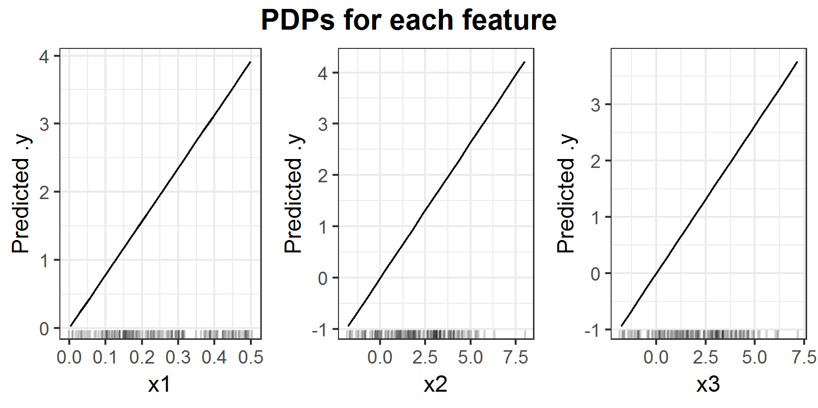
FIGURE 6.1: PDPs for prediction function \(f(x_1, x_2, x_3) = x_1 x_2 x_3\).

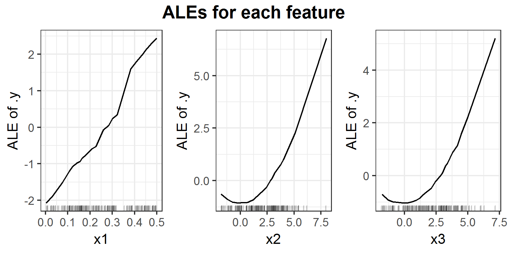
FIGURE 6.2: ALEs for prediction function \(f(x_1, x_2, x_3) = x_1 x_2 x_3\).

Plot 6.1 shows the 1D PDP for each of the three features. One can see that the PDP detects a linear influence on the prediction for all 3 of the features.

On the other hand, the ALE (figure 6.2) attests the linear influence to the feature \(x_1\) only. This plot exposes a weakness of the ALE compared to the PDP straight away. The ALE depends much more on the sampled data than the PDP does. The result is that the ALE can look a bit shaky. In this special case, it is that seriously one almost can't see the linear influence. If there would be more data or fewer intervals for the estimation, the plot would look more like the PDP for feature \(x_1\). The two other features seem to rather have a quadratic influence on the prediction. And this is the case indeed since it is the 'true' link between prediction and the correlated features. Feature \(x_3\) has (in expectation) the same value as \(x_2\). Especially if feature \(x_1\) has small values the variance of feature \(x_2\) around \(x_3\) becomes small as well. As consequence the last part of the prediction function '\(x_2 x_3\)' can be approximated by '\(x_2^2\)' or '\(x_3^2\)'. This explains the quadratic influence. By changing the prediction formula to \(f(x_1, x_2, x_3) = y = x_1 x_2^2\) the figures 6.3 and 6.4 for PDP and ALE plots are estimated.

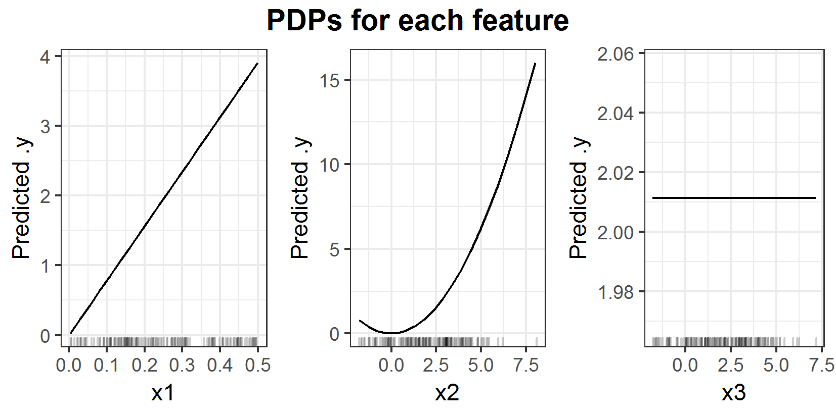
FIGURE 6.3: PDPs for prediction function \(f(x_1, x_2, x_3) = x_1 x_2^2\).

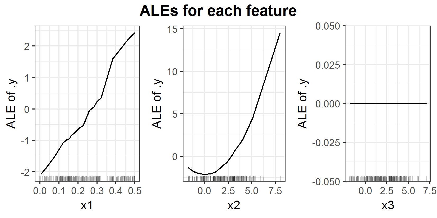
FIGURE 6.4: ALEs for prediction function \(f(x_1, x_2, x_3) = x_1 x_2^2\).

Plots 6.3 and 6.4 clearly show the linear influence of \(x_1\) again. Additionally this time both (ALE and PDP) attest a quadratic influence to feature \(x_2\) on the prediction. Since \(x_3\) does not have any influence on the prediction function, it is correct, that there is no influence detected. The reason for this behavior lies in the calculation method for the PDP. With the new prediction formula only depending on uncorrelated features \(x_1\) and \(x_2\), the PDP works well. Since now the approach of PDP to calculate the mean effect is correct.

6.1.2 Example 2: Additive prediction function

In this example, PDP and ALE will be applied to an additive prediction function.

A data set consisting of three features (\(x_1\), \(x_2\), \(x_3\)) is constructed. In this case the target variable is \(y = x_1 + x_2 - x_3\). Once again the prediction function is not learned but set to exactly the target variable, meaning \(f(x_1, x_2, x_3) = x_1 + x_2 - x_3\). The distributions are similar to the ones from example 1 and again 150 observations are sampled. \(X_1 \sim \mathcal{U}(0,~2)\), \(X_2 \sim \mathcal{N}(2,~0.5)\) and \(X_3\mid X_2 \sim \mathcal{N}(X_2,~0.5)\)

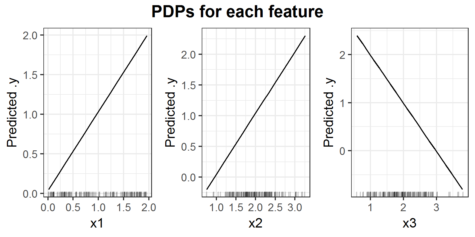
FIGURE 6.5: PDPs for prediction function \(f(x_1, x_2, x_3) = x_1 + x_2 - x_3\).

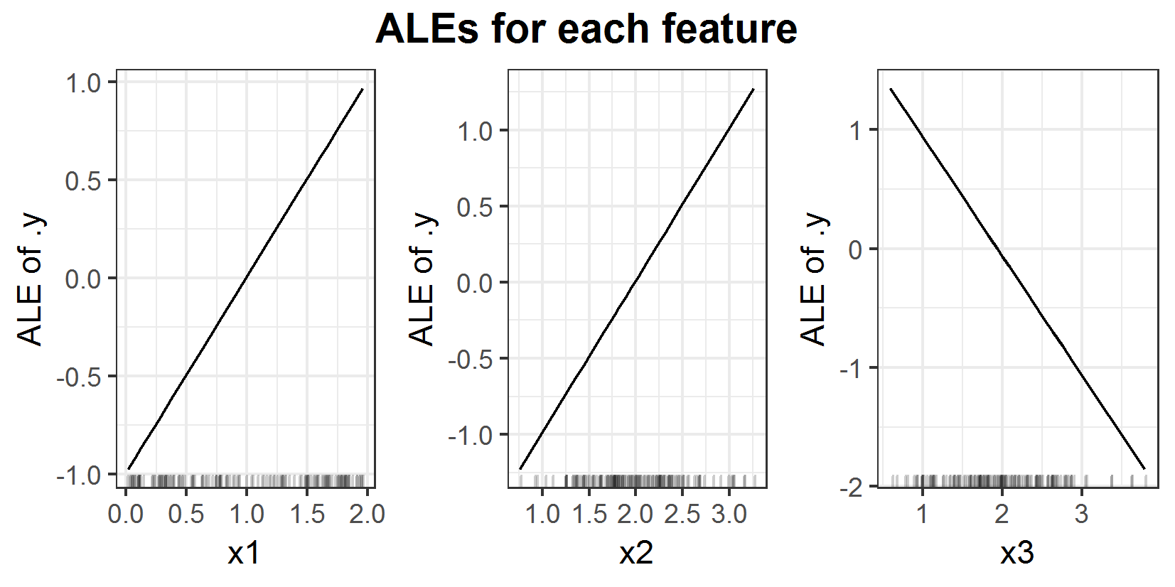
FIGURE 6.6: ALEs for prediction function \(f(x_1, x_2, x_3) = x_1 + x_2 - x_3\).

For this example one can see that the ALEs (6.6) and PDPs (6.5) are basically the same. Ignoring the centering both attest the same linear influence for all three features. And since it is an additive model this is actually correct. But neither the ALE nor the PDP recognize the strong correlation between the features \(x_2\) and \(x_3\). The real influence of features \(x_2\) and \(x_3\) is in expectation zero, since it is \(x_2 - x_3\) and \(E[X_3 \mid X_2] = X_2\). So \(E[X_2 - X_3 \mid X_2] = 0\).

This shows a few points one has to be aware of when working with these plots. In this example, if one uses the interpretation of the PDP for feature \(x_2\) and states 'If the value of feature \(x_2\) is 2.5, then I expect the prediction to be 1.5' it would be wrong. The problem here is the extrapolation in the estimation of the PDP. So it does not take into account any connection between the features but still works as good as the ALE in this example.

The general advantage of the ALE is the small chance of extrapolation in the estimation. But this does not mean it would recognize any correlation between the features in each scenario. And it is in general not possible to state something about the prediction with only one 1D ALE. The ALE is just showing the expected and centered main effect of the feature. In this example an interpretation like 'If feature \(x_2\) has value 2.5 then in expectation the prediction will be 0.5 higher than the average prediction' is wrong. If one needs a statement like that the other strongly correlated features have to be taken into account as well. One has to be aware of the higher order effects of the ALE, too.

To conclude the analysis of this example 2D ALEs are necessary. So it will be continued later this chapter.

6.2 Comparison two features

Before the 2D ALE and PDP will be applied to the same predictors, the 2D ALE has to be introduced. In the first place, the theoretical formula will be defined. Thereafter the estimation will be derived and then the comparison to the 2D PDP will be made.

6.2.1 The 2D ALE

6.2.1.1 Theoretical Formula 2D ALE

Similar to one variable of interest there is a theoretical formula for a 2-dimensional ALE. This ALE aims to visualize the 2nd order effect. Meaning one will just see the additional effect of interaction between those two features. The main effects of the features will not be shown in the 2D ALE.

To explain the formula it will be assumed that \(x_j\) and \(x_l\) are the two features of interest. The rest of the features is represented by \(x_c\). So in the following variable \(x_c\) can be of higher dimension than 1. As for the 1D ALE, there is again a theoretical derivative for the fitted function \(\hat{f}\). But this time it is the derivative in the direction of both features of interest. So in the following, this notation will hold:

\[ \hat{f}^{(j,~l)}(x_j,~x_l,~x_c) = \frac{\delta\hat{f}(x_j,~x_l,~x_c)}{\delta x_j~ \delta x_l}\]

The whole formula would be very long, so it is split into 3 parts (compare (Apley 2016, 8)):

1. The 2nd order effect (6.1)

2. 2nd order effect corrected for both main effects (6.2)

3. The 2D ALE; the corrected 2D ALE centered for its mean overall effect (6.3)

Equation (6.1) is the 2nd order effect with no correction for main effects of \(x_j\) and \(x_l\). So this is not yet the pure 2nd order effect the 2D ALE is aiming for.

\[\begin{equation} \widetilde{\widetilde{ALE}}_{\hat{f},~j,~l}(x_j, x_l) = \notag \end{equation}\] \[\begin{equation} \int_{z_{0,j}}^{x_j} \int_{z_{0,l}}^{x_l} E[\hat{f}^{(j,~l)}(X_j,~X_l,~X_c)\mid X_j = z_j,~X_l = z_l]~dz_l~dz_j \tag{6.1} \end{equation}\]

Now from the uncorrected 2nd order effect, the two main effects of both features on the uncorrected 2D ALE are subtracted (see equation (6.2)). In this way the main effects of \(x_j\) and \(x_l\) on the final \(ALE_{\hat{f},~j,~l}(x_j, x_l)\) are both zero (Apley 2016, 9). But be careful, this is not centering by a constant as in the one-dimensional ALE. This is a correction for the also accumulated main effects which of course vary in the directions of the features.

\[\begin{align} \widetilde{ALE}_{\hat{f},~j,~l}(x_j, x_l) = &\widetilde{\widetilde{ALE}}_{\hat{f},~j,~l}(x_j, x_l) \notag \\ &- \int_{z_{0,~j}}^{x_j} E[\frac{\delta\widetilde{\widetilde{ALE}}_{\hat{f},~j,~l}(X_j, X_l)}{\delta X_j}\mid X_j = z_j]~dz_j \notag \\ &- \int_{z_{0,~l}}^{x_l} E[\frac{\delta\widetilde{\widetilde{ALE}}_{\hat{f},~j,~l}(X_j, X_l)}{\delta X_l}\mid X_l = z_l]~dz_l \tag{6.2} \end{align}\]

Equation (6.3) shows the final (centered) 2D ALE. The subtraction in the formula is now the real centering to shift the 2nd order effect (corrected for the main effects) to zero with respect to the marginal distribution of \((X_j, ~ X_l)\).

\[\begin{equation} ALE_{\hat{f},~j,~l}(x_j, x_l) = \widetilde{ALE}_{\hat{f},~j,~l}(x_j, x_l) ~ - E[\widetilde{ALE}_{\hat{f},~j,~l}(X_j, X_l)] \tag{6.3} \end{equation}\]

In the appendix 6.5.1 one can find the calculation of the theoretical ALE for Example 1.

6.2.1.2 Estimation 2D ALE

Analogously to the 1D ALE in most cases, it is not possible to calculate the 2D ALE. It has to be estimated. These estimation formulas are pretty long and might be confusing, especially the indices. But there will be an explanation including a visualization as well to clarify the estimation method.

First, all variables have to be defined. The two features of interest are \(x_j\) and \(x_l\). The prediction function is \(\hat{f}(x_j, x_l, x_{\setminus\{j,~l\}})\), while \(x_{\setminus\{j,~l\}}\) represents all the rest of the features, so it can be of higher dimension than 1. The areas including data for feature \(x_j\) and \(x_l\) are divided into the same number of intervals, namely K. The intervals in \(x_j\) direction are separated by \(z_{k,j}\) for \(k \in \{0,...,K\}\). \(k_j(x_j)\) returns the interval number in which \(x_j\) lies. This holds for \(z_{m,l}\) and \(k_l(x_l)\) respectively in direction of \(x_l\). \(N_{\{j,~l\}}(k,m)\) is the crossproduct of the k-th and m-th interval (in \(x_j\) and \(x_l\) direction), so it is defined as \((z_{k-1,j}, z_{k,j}] \times (z_{m-1,j}, z_{m,j}]\). \(n_{\{j,~l\}}(k,m)\) is the number of observations lying in this \(N_{\{j,~l\}}(k,m)\) cell. The parameter i represents the i-th observation (Apley 2016). With these variables in mind, the definition of the 2D ALE estimation can begin.

The estimation equvalent to Formula (6.1) is:

\[\begin{equation} \widehat{\widetilde{\widetilde{ALE}}}_{\hat{f},~j,~l}(x_j, ~x_l) = \notag \end{equation}\] \[\begin{equation} \sum_{k=1}^{k_j(x_j)} \sum_{m=1}^{k_l(x_l)} \frac{1}{n_{\{j,~l\}}(k,m)}\sum_{i:~x_{\{j,~l\}}^{(i)}\in N_{\{j,~l\}}(k,m)} ~ \Delta_{\hat f}^{{\{j,~l\}}, ~k,~m} (x_{\setminus\{j,~l\}}^{(i)}), \tag{6.4} \end{equation}\]

while the \(\Delta\) function is:

\[\begin{equation} \Delta_{\hat f}^{{\{j,~l\}}, ~k,~m} (x_{\setminus\{j,~l\}}^{(i)}) = \notag \end{equation}\] \[\begin{equation} [\hat f(z_{k,~j},~ z_{m,~l}, ~x_{\setminus\{j,~l\}}^{(i)}) - \hat f(z_{k-1,~j},~ z_{m,~l}, ~x_{\setminus\{j,~l\}}^{(i)})] \notag \end{equation}\] \[\begin{equation} - [\hat f(z_{k,~j},~ z_{m-1,~l}, ~x_{\setminus\{j,~l\}}^{(i)}) - \hat f(z_{k-1,~j},~ z_{m-1,~l}, ~x_{\setminus\{j,~l\}}^{(i)})] \tag{6.5} \end{equation}\]

Now the correction for the main effects (equation (6.6) corresponding to theoretical formula (6.2)) is estimated:

\[\begin{align} \widehat{\widetilde{ALE}}_{\hat{f},~j,~l}(x_j, ~x_l) = &\widehat{\widetilde{\widetilde{ALE}}}_{\hat{f},~j,~l}(x_j, ~x_l) \notag \\ &- \sum_{k=1}^{k_j(x_j)} \frac{1}{n_j(k)} \sum_{m=1}^{K} ~ n_{\{j,~l\}}(k,m) [\widehat{\widetilde{\widetilde{ALE}}}_{\hat{f},~j,~l}(z_{k,~j}, ~z_{m,~l}) \notag \\ &~~~~~~~~~~~~~~~~~~~~~~~ - \widehat{\widetilde{\widetilde{ALE}}}_{\hat{f},~j,~l}(z_{k-1,~j}, ~z_{m,~l})]\notag \\ &- \sum_{k=1}^{k_l(x_l)} \frac{1}{n_l(k)} \sum_{m=1}^{K} ~ n_{\{j,~l\}}(k,m) [\widehat{\widetilde{\widetilde{ALE}}}_{\hat{f},~j,~l}(z_{k,~j}, ~z_{m,~l}) \notag \\ &~~~~~~~~~~~~~~~~~~~~~~~ - \widehat{\widetilde{\widetilde{ALE}}}_{\hat{f},~j,~l}(z_{k,~j}, ~z_{m-1,~l})] \tag{6.6} \end{align}\]

Equation (6.6) is the uncentered 2D ALE since it is just corrected for its main effects. And this is not a real centering in the sense of subtracting a constant value. Now it will be centered for its estimation \(E[\widehat{\widetilde{ALE}}_{\hat{f},~j,~l}(X_j, ~X_l)]\) and this is a constant, so there will be no effect on the general shape of the ALE plot. Again this expected value has to be estimated, to complete the 2D ALE as is calculated in theoretical formula (6.3).

\[\begin{equation} \widehat{ALE}_{\hat{f},~j,~l}(x_j, ~x_l) = \notag \end{equation}\] \[\begin{equation} \widehat{\widetilde{ALE}}_{\hat{f},~j,~l}(x_j, ~x_l) - \sum_{k=1}^{K}\sum_{m=1}^{K} ~ n_{\{j,~l\}}(k,m) ~ \widehat{\widetilde{ALE}}_{\hat{f},~j,~l}(z_{k,~j}, ~z_{m,~l}) \tag{6.7} \end{equation}\]

In contrast to the ALE for one feature of interest, the 2D ALE ((6.7) is a two-dimensional step function, so there is no smoothing or something similar to make it a continuous function.

These formulas are pretty long, so to get an intuition of the estimation figure 6.7 will be helpful.

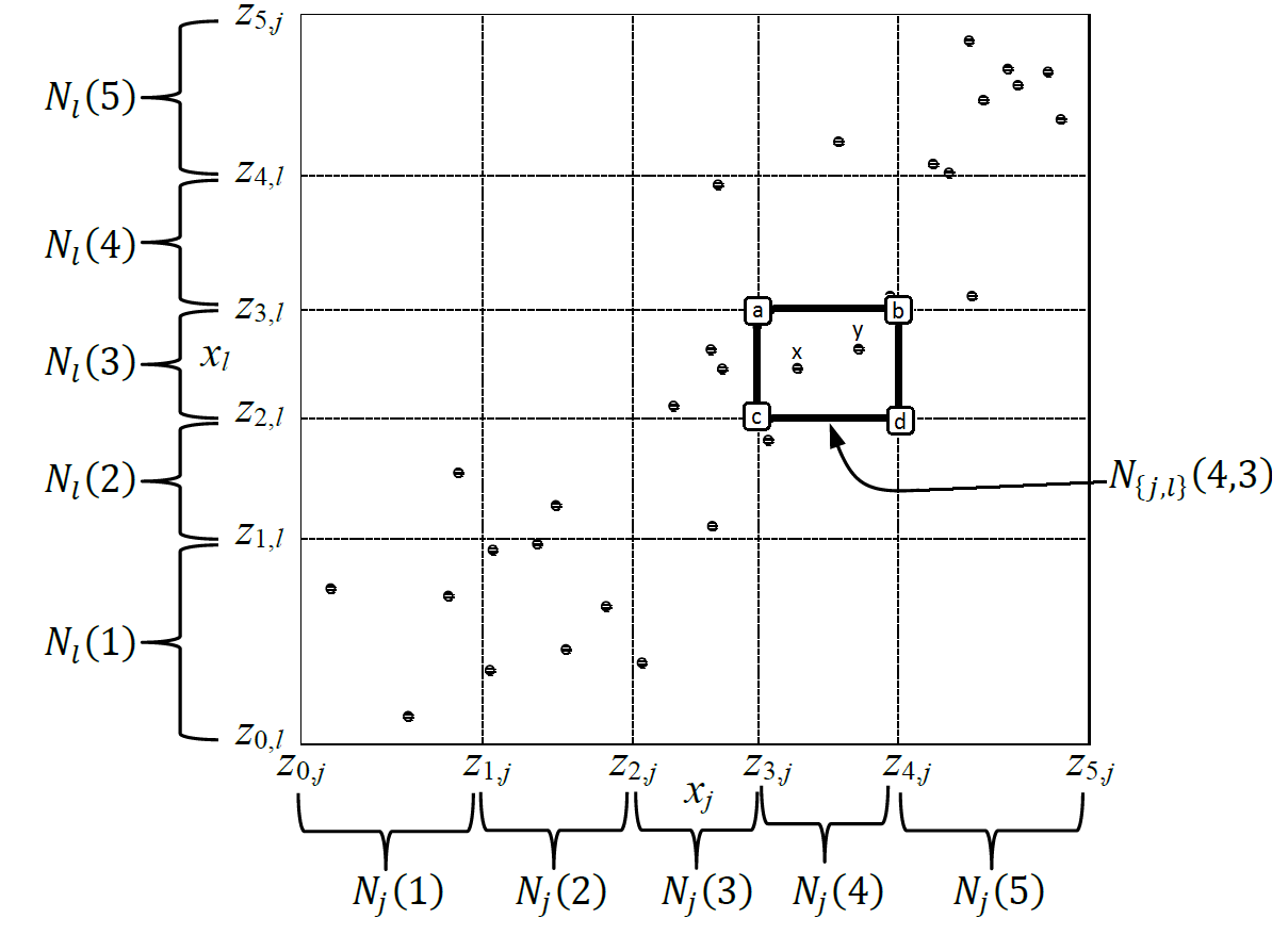
FIGURE 6.7: Visualization of the absolut differences for the 2nd order effect (Apley 2016, 13) and (Molnar 2019).

To calculate the delta (6.5) for the uncorrected and uncentered ALE estimation in each cell the predictions for the data points in that cell will be calculated pretending the \(x_l\) and \(x_j\) values are the corner values of the cell they are in. In the case of figure 6.7, these 2-dimensional corner values would be a, b, c, d. The delta for point x in this example would be calculated like this:

\[\begin{align} \Delta_{\hat f}^{{\{j,~l\}}, ~4,~3} (x_{\setminus\{j,~l\}}) = & [\hat f(b, ~x_{\setminus\{j,~l\}}) - \hat f(a, ~x_{\setminus\{j,~l\}})] \notag \\ &- [\hat f(d, ~x_{\setminus\{j,~l\}}) - \hat f(c, ~x_{\setminus\{j,~l\}})] \notag \end{align}\]

The same would be done for point y. Thereafter the deltas would be averaged to get the mean delta for cell \(N_{\{j,~l\}}(4,3)\). This would then be accumulated over all cells left or beneath this cell to get the uncorrected and uncentered ALE for the values in \(N_{\{j,~l\}}(4,3)\).

The correction for the main effects extracts the pure 2nd order effect for the two features of interest by subtracting the main effect of the single features on the ALE (equation (6.6)). To stick with this example the correction for the main effect of feature \(x_j\) for values in \(N_j(4)\) takes into account all cells in the first 4 columns and aggregates the first order effect. In cell \(N_{\{j,~l\}}(4,3)\) this would look like this:

\[ \widehat{\widetilde{\widetilde{ALE}}}_{\hat{f},~j,~l}(b) - \widehat{\widetilde{\widetilde{ALE}}}_{\hat{f},~j,~l}(a)\]

The correction for \(x_l\) looks pretty much the same just from the other direction. It takes into account the first 3 rows. So in cell \(N_{\{j,~l\}}(4,3)\) the first order effect in direction of \(x_l\) would be

\[ \widehat{\widetilde{\widetilde{ALE}}}_{\hat{f},~j,~l}(b) - \widehat{\widetilde{\widetilde{ALE}}}_{\hat{f},~j,~l}(d). \]

Thereafter the corrected ALE is centered for its mean (equation (6.7)), pretty much the same way as is done for one dimension. But this time the aggregation is not just over a line but over a grid.

There are a few questions that might arise.

First, how is the grid for the estimation defined? In the iml package, the cells are the cross products of the intervals used for the 1D estimation. It would be very hard to make a grid of rectangles which all include roughly the same amount of data points.

Another question is: How does the estimation treat empty cells, which include no data points? There are two options, they can either be ignored and greyed out or they receive the value of their nearest neighbor rectangle, which is determined using the center of the cells. The last method is implemented in the iml package. This happens right after averaging over the \(\Delta_{\hat f}^{{\{j,~l\}}, ~k,~m} (x_{\setminus\{j,~l\}})\)s before the correction for the 1st order effects is done.

6.2.1.3 Example 1 continued - Theoretical and estimated 2D ALE

Before ALE and PDP will be compared for two features of interest, the analysis of example 1 will be continued in two dimensions, to get a first glance at the 2D ALE.

The data set is basically the same, just for sake of clearness in the 2D ALE example the distributions are a bit different. A data set consisting of 150 observations with three features (\(x_1\), \(x_2\), \(x_3\)) and the prediction function \(f(x_1, x_2, x_3) = x_1 x_2 x_3\) is considered. But this time the three features are sampled from these disrtibutions: \(X_1 \sim \mathcal{U}(0,~0.5)\), \(X_2 \sim \mathcal{N}(5,~1)\) and \(X_3\mid X_2, X_1 \sim \mathcal{N}(X_2,X_1)\). So feature \(x_2\) is expected to be 5 and has a lower variance than it has in example 1. The rest stays the same.

With the formulas in the appendix 6.5.1 it is possible to calculate the theoretical 2D ALE.

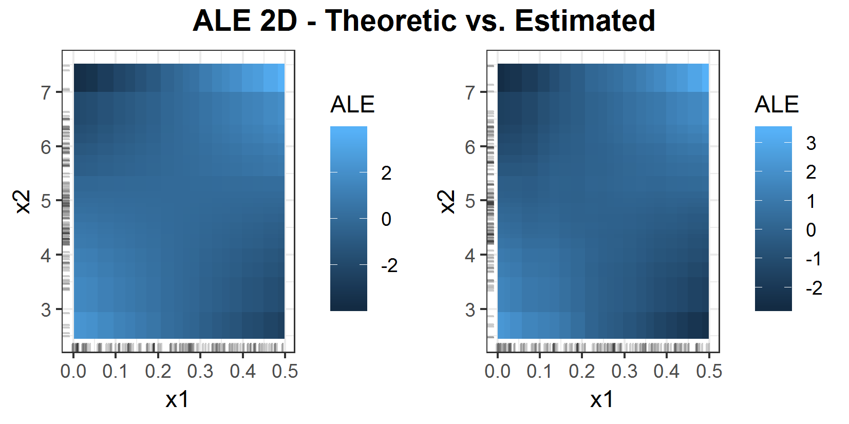
FIGURE 6.8: Theoretical 2D ALE (left) and estimated ALE (right).

Figure 6.8 shows the theoretical ALE compared to the estimated one. In this example, it looks pretty similar. The interpretation is a bit hard. Since one can only see the 2nd order effects, isolated from the 1st order effects, it is hardly possible to state something reasonable about the prediction with just this plot. But this problem will be discussed in the coming up chapter.

6.2.2 2D ALE vs 2D PDP

In this Chapter, only 2D plots for artificially constructed examples will be analyzed. To show the statement, that there are no main effects in the 2D ALE example 2 will be discussed again.

6.2.2.1 Example 2 - 2D comparison

Just a short reminder of example 2: the prediction function here is \(f(x_1, x_2, x_3) = x_1 + x_2 - x_3\) and \(x_2\) and \(x_3\) are strongly positive correlated (they even share the same expected value).

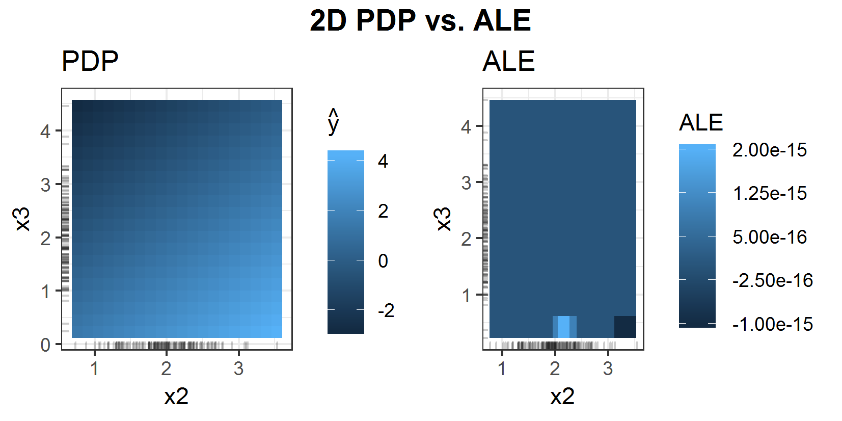
FIGURE 6.9: 2D PDP (left) vs. 2D ALE (right) for prediction function \(f(x_1, x_2, x_3) = x_1 + x_2 - x_3\).

Figure 6.9 shows the direct comparison of 2D PDP and 2D ALE. The ALE is almost completely zero as expected. In this additive example, there are main effects only and since the 2D ALE is corrected for the main effects of the features, there is no pure 2nd order effect. The PDP in comparison shows the mean prediction. So, of course, there are the main effects estimated within the 2D PDP as well. Obviously, it is hard to compare those two interpretation algorithms just like this.

To get a better comparison the main effects (1D ALEs) of the two features of interest can be added to the 2D ALE.

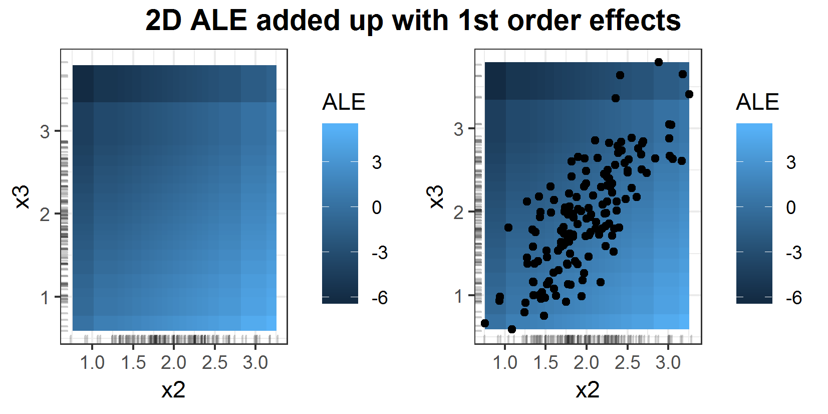
FIGURE 6.10: 2D ALE added up with 1st order effects of features \(x_2\) and \(x_3\) for prediction function \(f(x_1, x_2, x_3) = x_1 + x_2 - x_3\). In the right plot the underlying 2 dimensional data points are included.

Plot 6.10 shows the ALE added up with the corresponding 1st order effects of the features. And now it seems pretty much the same as the PDP in figure 6.9. On the right side, the same plot can be seen. This one additionally includes the underlying data points regarding features \(x_2\) and \(x_3\). Furthermore these two features are independent of feature \(x_1\), so the PDP and ALE yield the same correct interpretation, namely for realistic data points the influence of these two features is close to zero because of their strong positive correlation and their opposing first order effects (figures 6.6 and 6.5).

With this in mind, example 1 deserves another look regarding the 2nd order effect in comparison to the PDP.

6.2.2.2 Example 1 - 2D comparison

To be able to compare the 2D ALE from the last chapter for prediction function \(f(x_1, x_2, x_3) = x_1 x_2 x_3\) with the 2D PDP one also should add up the 1st order effects to the 2D ALE.

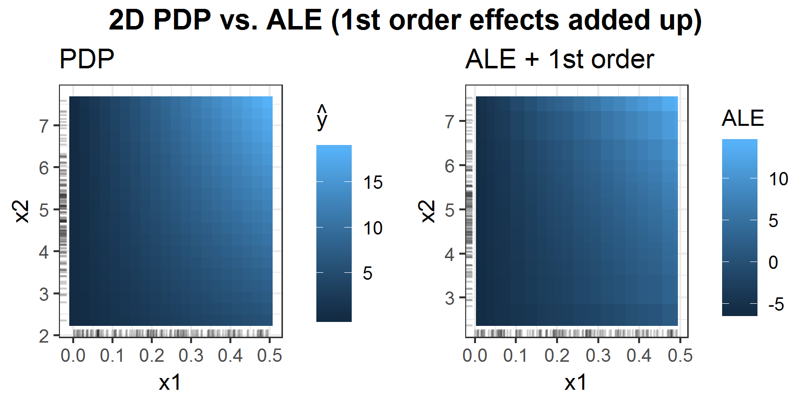
FIGURE 6.11: 2D PDP vs 2D ALE with added up 1st order effects of features \(x_1\) and \(x_2\) for prediction function \(f(x_1, x_2, x_3) = x_1 x_2 x_3\).

This plot 6.11 shows exactly what happens in this case, when the 1st order effects of the ALE are added up to the 2nd order effects. One can see that although the connection between \(x_2\) and \(x_3\) has been detected by the 1st order ALEs (figure 6.2) and has not been by the 1D PDPs (figure 6.1), the comparable 2D plots look pretty much the same.

In these two examples, it seems like the 2D ALE is not much better than the 2D PDP. But making just a small change to the prediction function for unrealistic values (regarding the underlying data) exposes the sensitivity of the PDP estimation for extrapolation.

6.2.2.3 Example 1 modified - 2D comparison

The setting of the problem stays basically the same. Just a small - for the real prediction actually irrelavant - change is made for the prediction function. It is not anymore \(f(x_1, x_2, x_3) = x_1 x_2 x_3\) but

\[ f(x_1, x_2, x_3) = \begin{cases} x_3^3, \quad\quad\quad\quad\quad~~\text{if}~x_3\ge6 ~~, ~~x_2\le4\\ x_1 x_2 x_3, \quad\text{else}\\ \end{cases} \] This seems a bit unrealistic but especially tree-based predictors tend to do 'strange' things in areas without data.

The result of the 2D PDP compared to the ALE (figure 6.12) shows the problem. In the area where \(x_2 < 4\) the values of the PDP are huge, since the big values for \(x_3^3\) if \(x_3 > 6\) increase the average drastically. These values are very unlikely for the underlying distribution but the PDP pretends them to be possible. This is the problem of the extrapolation in the PDP estimation. This is not a problem for the ALE. Here one can not recognise any difference to figure 6.11, where the prediction function is just \(f(x_1, x_2, x_3) = x_1 x_2 x_3\).

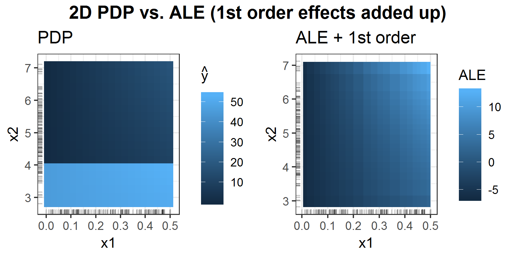
FIGURE 6.12: 2D PDP vs 2D ALE with added up 1st order effects of features \(x_1\) and \(x_2\) for stepwise prediction function.

One big advantage of the ALE in general over the PDP is, that it hardly extrapolates in the estimation, which is usually the case for the PDP with correlated features. And one can take a look at separated 1st and 2nd order effects, which can be very helpful, especially for real black box models with complicated links. Furthermore, in the next chapter, the runtime will turn out to be a strong advocate for the ALE, especially for bigger datasets.

6.3 Runtime comparison

In this chapter, the runtime of ALE and PDP will be compared. Therefore three general sizes of data sets have been sampled. One small with 100, a bigger one with 1,000 and the biggest with 10,000 observations. The number of features varies between 5 and 40, while there are always 2 categorial features and the others are numeric, as is the target variable. The predictor applied to these datasets is a regular SVM. It is way faster than the random forest, where the PDP estimation can easily take half a minute for just 1,000 observations.

To compare the runtime, the package 'microbenchmark' has been used. So the discussed results will all have the same structure, which will be explained with the first example. The comparison will cover the runtime for...

1. ...one numerical feature of interest
2. ...two numerical features of interest
3. ...one categorial feature of interest.

Each of these three will be compared for the different numbers of observations of course but also for different grid sizes (number of intervals the ALE and PDP are estimated on) and varying feature numbers.

6.3.1 One numerical feature of interest

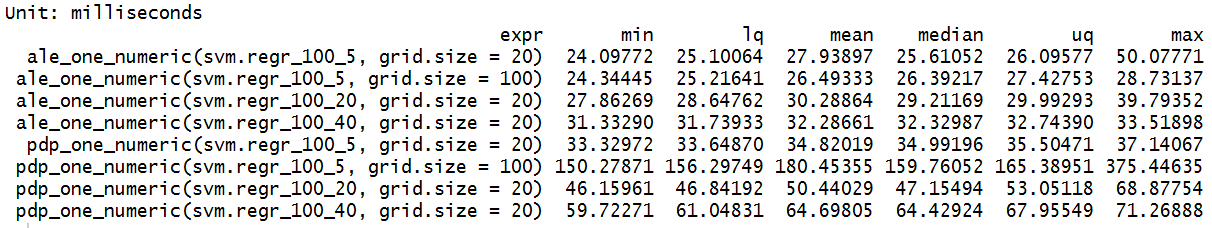
FIGURE 6.13: Runtime comparison ALE vs. PDP for one numeric feature. Differences for the number of features and grid size.

Figure 6.13 shows the runtimes for different configurations in milliseconds. The microbenchmark output shows the compared expressions (here the calculation of ALE and PDP) in the first column. The other columns are the measured runtime for 10 different runs. From left to right it is the minimum runtime, the lower quantile of the runtimes, the mean, the median, the upper quantile, and the maximal runtime. The main attention usually lies in the mean. In the expression, there are also configurations for the sampled dataset integrated. For example 'ale_one_numeric(svm.regr_100_5, grid.size = 20)' represents the following estimation: An ALE for one numeric feature of interest has been estimated. The prediction function was an SVM, fitted and evaluated on a sample of 100 observations with 5 features. The grid size, in this case, was 20, so the plots are estimated on 20 intervals.

Plot 6.13 shows the comparison for a change in grid size and number of features for one numeric feature of interest. It seems like the number of features does barely influence the runtime. Additionally for the ALE the grid size is not significantly changing the runtime.

That is completely different for the PDP. Here a factor 5 for the number of intervals increases the runtime by the same factor. This can be derived from the estimation. The ALE does the same number of predictions for any number of intervals, namely #observaions \(\times\) 2. It just averages more often for more intervals. But that happens without the prediction function and is just a simple mean calculation, so it barely needs time. The PDP, on the other hand, estimates the mean prediction for each interval border. So here (#intervals + 1) \(\times\) #observations predictions have to be calculated. So the runtime grows linearly with the grid size and factor #observations. This is also the explanation for the next comparison (figure 6.14). Here again, one can see a way faster increase of runtime for PDPs than for ALEs when increasing the number of observations

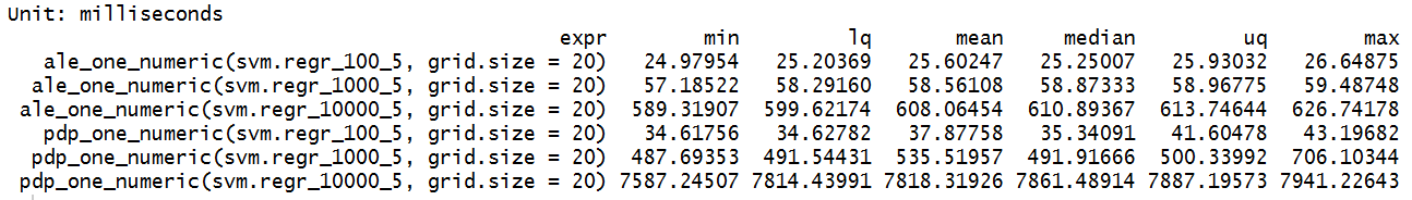
FIGURE 6.14: Runtime comparison ALE vs. PDP for one numeric feature. Differences for the number of observations.

6.3.2 Two numerical features of interest

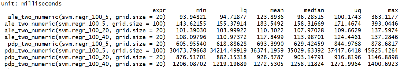
FIGURE 6.15: Runtime comparison ALE vs. PDP for two numeric features. Differences for number of features and grid size.

In figure 6.15 the runtimes for different 2D ALE and PDP configurations can be seen. Again the number of features is not a great deal for both algorithms. The ALE has no huge increase in runtime when the grid size is higher but the PDP has. The issue here is that the estimation for 2D PDP requires \((grid.size + 1)^2 \times \#observations\) predictions, while the ALE just needs \(4 \times \#observations\) predictions calculated for the estimation. This especially can be seen when increasing the number of observations.

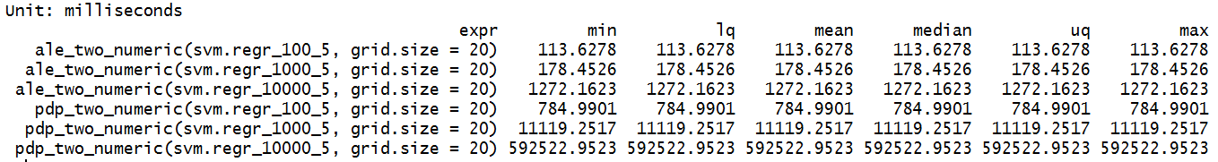
FIGURE 6.16: Runtime comparison ALE vs. PDP for two numeric features. Differences for the number of observations.

Figure 6.16 shows such an increase in observations. One can see that factor 100 in observations becomes almost factor 1,000 for the runtime of PDP while it is just a bit more than 10 for ALE.

6.3.3 One categorial feature of interest

Lastly, a look at the estimation for 1D categorial PDP and ALE will be taken.

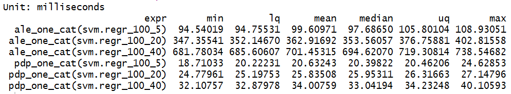
FIGURE 6.17: Runtime comparison ALE vs. PDP for one categorial feature. Differences for number of features only, since there is no grid size for categorial features.

Figure 6.17 shows the runtimes of PDP and ALE for a categorial feature of interest. Analyzing categorial features does not require a grid size since the number of categories already defines the number of different evaluations. This time one recognizes that it is the other way around. The calculation time stays the same for the PDP with a growing number of features, while ALE shows a significant growth. This is clearly caused by the reordering of the features for their category (will be explained in the next chapter). The reordering is based on the kind of nearest neighbors (depends on implementation). The calculation of these neighbors takes longer the more features have to be taken into account.

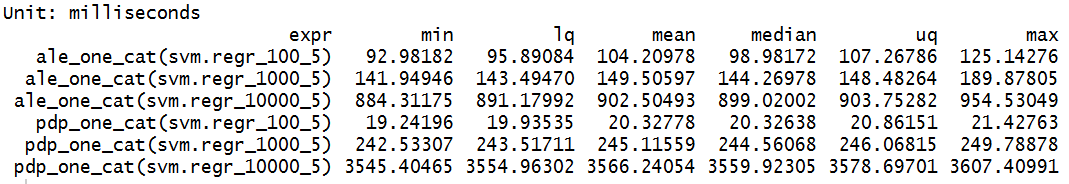
FIGURE 6.18: Runtime comparison ALE vs. PDP for one categorical feature. Differences for the number of observations.

Figure 6.18 shows a similar picture as can be seen in figure 6.13. Just this time compared to the estimation for one numeric feature the ALE is way slower for the categorial feature, while the PDP is twice as fast as for the numeric feature. That might come from the fact that the grid size here (6.13) was 20 and in this case, there are just 10 classes for the feature of interest. Meaning that half as many calculations for the estimation are required. So it might be the same speed for the PDP from numeric to categorial (at least with comparable parameters). The ALE will always be slower for categorical features since the reordering of the categories is necessary.

In general, one can state that ALE is by far faster. For an SVM that might not be that much of a problem. But with ensemble predictors like a random forest it can be very slow to calculate a PDP for a high grid size and 10,000+ observations.

6.4 Comparison for unevenly distributed data - Example 4: Munich rents

To conclude this chapter a real-world problem with a fitted learner will be analyzed with ICE, PDP, and ALE, to see them in action.

This is an example with data for rents in Munich from 2003. The target variable 'nm' is the rent per month per flat. To predict the rent a random forest has been fitted. The features in this example are 'wfl' (size in square meters) and 'rooms' (number of rooms) of the flat. These two variables are clearly positively correlated since there will not be an apartment with 15 square meters and 5 rooms. The other features are not that strongly correlated as one can see in figure 6.19. To fit the random forest only 'wfl' and 'rooms' were used.

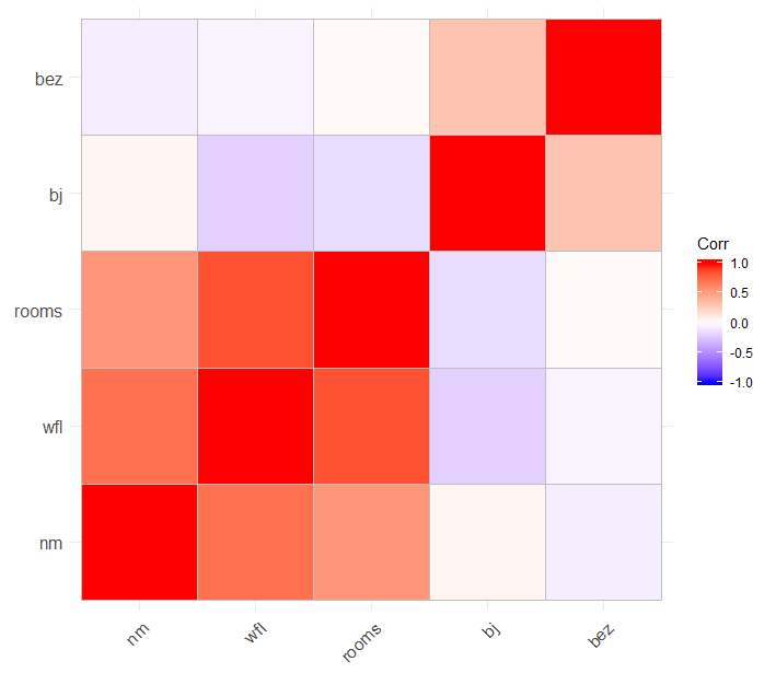
FIGURE 6.19: Correlation matrix for rents in Munich.

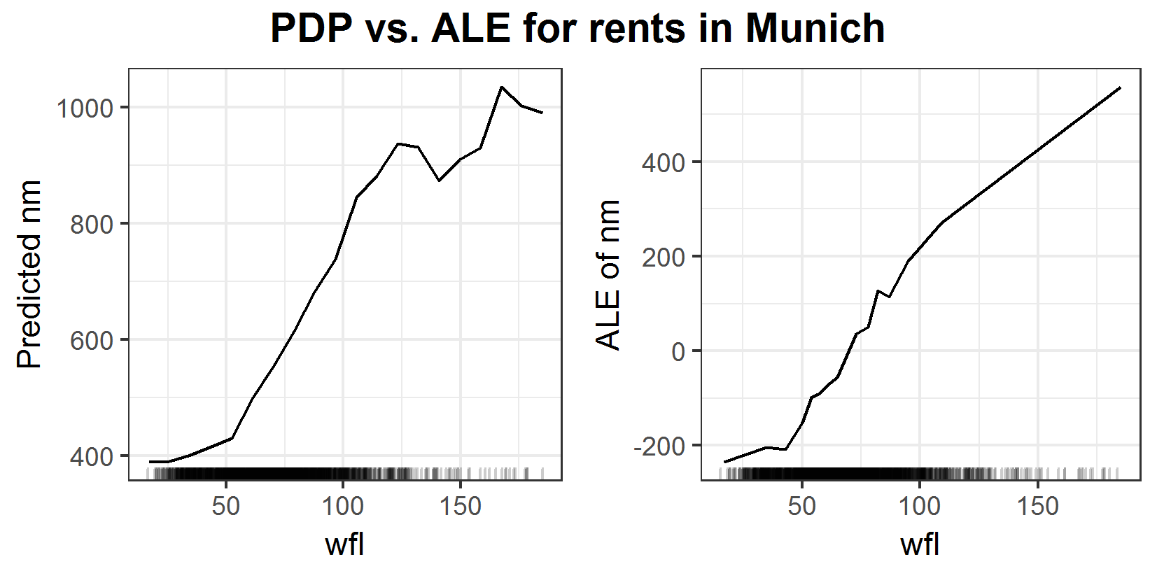
FIGURE 6.20: PDP and ALE plots for the influence of space on rents in Munich.

Figure 6.20 shows a more or less expected influence of space on the rent. The bigger the apartment the more expensive it is. In the area with a lot of data between 0 and 100, the PDP looks more smooth than the ALE which is a bit shaky. In the area with not that many observations, it is the other way around. The PDP suddenly breaks down what seems quite unrealistic, while the ALE has a pretty straight trend. Since the ALE shows a more expected behavior for the prediction of rents one could tend to state that the ALE outperforms the PDP. One could think that some unrealistic feature combinations in the estimation of the PDP caused this strange drop. But a look at the ICE plot reveals something else.

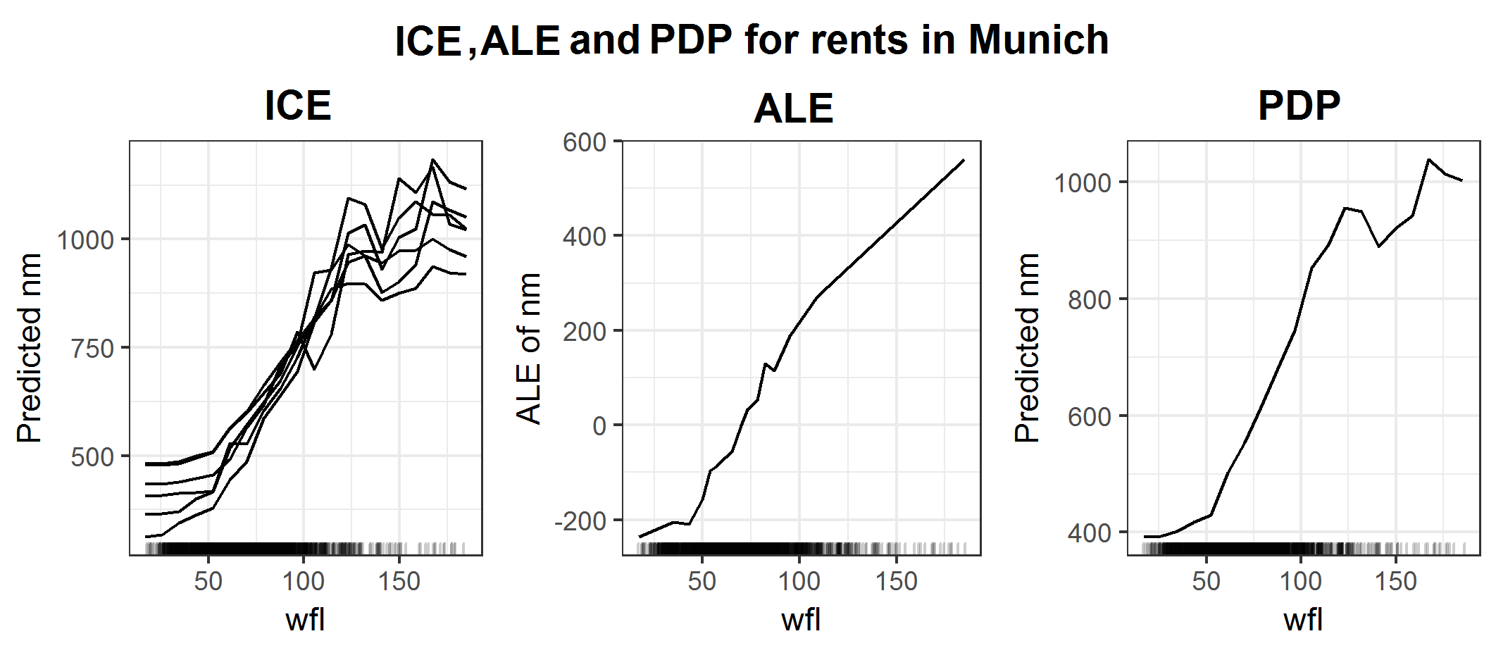
FIGURE 6.21: ICE, ALE and PDP plots for influence of space on rents in Munich.

Figure 6.21 additionally shows the ICE curves for this example. Since the only other feature used for the fit was 'rooms' and in the data set are just flats with 6 or fewer rooms, there are just 6 graphs. Now one could argue, maybe the apartments with less than 4 rooms (which are way more in this data set than those with 4 or more rooms) somehow cause the strange drop for the PDP. But figure 6.22 shows that almost all rooms have this drop, especially the apartments with 4 and 5 rooms.

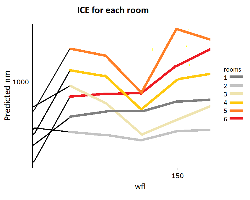
FIGURE 6.22: ICE for rents in Munich zoomed in for the critical area.

The issue here is that rooms don't have a strong influence on the prediction at all. In return, the PDP does not get problems with the correlation between the two features. And the PDP in the iml implementation generates an equidistant grid on the area with observations for feature 'wfl'. On the other hand, the ALE divides this area aiming for equally many observations in each interval. This results in very small intervals for apartments with less than 109 square meters of space. But the flats with 109 or more square meters are evaluated in one interval only. This simply yields to this ALE plot, where it just ignores/skips this drop. And as one can see this can be dangerous when interpreting the prediction function. In this special situation, the ALE might get better the true link between the rent and the size of the apartments but that is not what one is interested in. The goal is always to interpret the predictor and not the data.

This example demonstrated a crucial weakness of the ALE regarding the size of the intervals, which will be discussed in the next chapter. It also shows that ICE and PDP might still be worth a look despite their issues with correlated features and runtime. In general, if one needs to get a deep understanding of the prediction function it might be clever to use as many interpretation algorithms as possible. By being aware of their strengths and weaknesses and combining the results of those algorithms one can get a detailed look at the influence of each variable which should also be reliable.

6.5 Appendix

6.5.1 Calculation of theoretical 2D ALE example

Features \(x_1\), \(x_2\), \(x_3\) and the prediction function \(\hat{f}(x_1, x_2, x_3) = x_1 x_2 x_3\) are given. The features are sampled from the these disrtibutions: \(X_1 \sim \mathcal{U}(a,~b)\), \(X_2 \sim \mathcal{N}(\mu,~\sigma)\) and \(X_3\mid X_2, X_1 \sim \mathcal{N}(X_2,X_1)\).

The theoretical 2D ALE for features \(x_1\) and \(x_2\) will be calculated.

First is the calculation of uncorrected and uncentered 2nd order effect:

\[\begin{align} \widetilde{\widetilde{ALE}}_{\hat{f},~1,~2}&(x_1, x_2) = \notag \\ &= \int_{z_{0,1}}^{x_1} \int_{z_{0,2}}^{x_2} E[\hat{f}^{(1,~2)}(X_1,~X_2,~X_3)\mid X_1 = z_1,~X_2 = z_2]~dz_2~dz_1 \notag \\ &= \int_{z_{0,1}}^{x_1} \int_{z_{0,2}}^{x_2} E[X_3 \mid X_1 = z_1,~X_2 = z_2]~dz_2~dz_1 \notag \\ &= \int_{z_{0,1}}^{x_1} \int_{z_{0,2}}^{x_2} z_2 ~dz_2~dz_1 \notag \\ &= \int_{z_{0,1}}^{x_1} \frac{1}{2} (x_2^2 - z_{0,~2}) ~dz_1 \notag \\ &= \frac{1}{2} (x_2^2 - z_{0,~2})~(x_1 - z_{0,~1}) \end{align}\]

Next is the calculation of the corrected pure 2nd order effect:

\[\begin{align} \widetilde{ALE}_{\hat{f},~1,~2}(x_1, x_2) = ~ &\widetilde{\widetilde{ALE}}_{\hat{f},~1,~2}(x_1, x_2) \notag \\ & ~ - \int_{z_{0,~1}}^{x_1} E[\frac{\delta\widetilde{\widetilde{ALE}}_{\hat{f},~1,~2}(X_1, X_2)}{\delta X_1}\mid X_1 = z_1]~dz_1 \notag \\ & ~ - \int_{z_{0,~2}}^{x_2} E[\frac{\delta\widetilde{\widetilde{ALE}}_{\hat{f},~1,~2}(X_1, X_2)}{\delta X_2}\mid X_2 = z_2]~dz_2 \tag{6.8} \end{align}\]

The two terms which are correcting for the main effect of the two features will be calculated seperately:

\[\begin{align} \int_{z_{0,~1}}^{x_1} E[\frac{\delta\widetilde{\widetilde{ALE}}_{\hat{f},~1,~2}(X_1, X_2)}{\delta X_1} & \mid X_1 = z_1]~dz_1 = \notag \\ &= \int_{z_{0,~1}}^{x_1} E[\frac{1}{2}(X_2^2 - z_{0, ~2}^2)\mid X_1 = z_1]~dz_1 \notag \\ &= \int_{z_{0,~1}}^{x_1} \frac{1}{2}(\mu^2 + \sigma^2 - z_{0,~2}^2) ~dz_1 \notag \\ &= \frac{1}{2}(\mu^2 + \sigma^2 - z_{0,~2}^2)~(x_1 - z_{0,~1}) \tag{6.9} \end{align}\] \[\begin{align} \int_{z_{0,~2}}^{x_2} E[\frac{\delta\widetilde{\widetilde{ALE}}_{\hat{f},~1,~2}(X_1, X_2)}{\delta X_2} &\mid X_2 = z_2]~dz_2 = \notag \\ &= \int_{z_{0,~2}}^{x_2} E[X_2 (X_1 - z_{0, ~1})\mid X_2 = z_2]~dz_2 \notag \\ &= \int_{z_{0,~2}}^{x_2} z_2(\frac{a+b}{2} - z_{0, ~1}) ~dz_2 \notag \\ &= \frac{1}{2}(\frac{a+b}{2} - z_{0, ~1})(x_2^2 - z_{0, ~2}^2) \tag{6.10} \end{align}\]

Combining (6.9) and (6.10) with (6.8) yields:

\[\begin{align} \widetilde{ALE}_{\hat{f},~1,~2}(x_1, x_2) &= \widetilde{\widetilde{ALE}}_{\hat{f},~1,~2}(x_1, x_2) - \frac{1}{2}(\mu^2 + \sigma^2 - z_{0,~2}^2)~(x_1 - z_{0,~1}) \notag \\ & ~~~ - \frac{1}{2}(\frac{a+b}{2} - z_{0, ~1})(x_2^2 - z_{0, ~2}^2) \notag \\ &= x_2^2~x_1 + (x_1 - z_{0,1})(\mu^2+\sigma^2) - \frac{a + b}{2}(x_2^2-z_{0,~2}^2) \end{align}\]

The last part is the centering for the mean:

\[\begin{align} ALE_{\hat{f},~1,~2}(x_1, x_2) &= \widetilde{ALE}_{\hat{f},~1,~2}(x_1, x_2) ~ - E[\widetilde{ALE}_{\hat{f},~1,~2}(X_1, X_2)] \notag \\ &= \frac{1}{2} (x_2^2~x_1 + (x_1 - z_{0,1})(\mu^2+\sigma^2) - \frac{a + b}{2}(x_2^2-z_{0,~2}^2) \notag \\ & ~~ - E[X_2^2~x_1 + (X_1 - z_{0,1})(\mu^2+\sigma^2) - \frac{a + b}{2}(X_2^2-z_{0,~2}^2)] ) \notag \\ &= \frac{1}{2} [x_2^2~x_1 - (x_1 - z_{0,1})(\mu^2+\sigma^2) - \frac{a + b}{2}(x_2^2-z_{0,~2}^2) \notag \\ & ~~ - (z_{0,1}(\mu^2+\sigma^2) + z_{0,~2}^2 \frac{a + b}{2} - (\mu^2+\sigma^2) \frac{a + b}{2}) ] \notag \\ &= \frac{1}{2} [x_2^2~x_1 - x_1(\mu^2+\sigma^2) - x_2^2 \frac{a + b}{2} + (\mu^2+\sigma^2) \frac{a + b}{2} ] \end{align}\]

This formula was used to calculate the theoretical plot in figure 6.8.

References

Apley, Daniel W. 2016. Visualizing the Effects of Predictor Variables in Black Box Supervised Learning Models. https://arxiv.org/ftp/arxiv/papers/1612/1612.08468.pdf.

Molnar, Christoph. 2019. Interpretable Machine Learning: A Guide for Making Black Box Models Explainable.