Chapter 11 PFI: Training vs. Test Data
Author: Cord Dankers
Supervisor: Florian Pfisterer
In this chapter we will deal with the question whether we should use test or training data to calculate permutation feature importance. First of all we'll give a short overview of the interesting components.
Permutation Feature Importance (PFI)
In order to calculate the impact of a single feature on the loss function (e.g. MSE), we shuffle the values for one feature to break the relationship between the feature and the outcome. Chapter \(8\) contains an introduction to permutation feature importance.
Dataset
In this chapter, we consider two partitions of a dataset \(D\):
\(D_{train}\): Training data, used to set up the model. Overfitting and underfitting is possible
\(D_{test}\): Test data used to check if the trained model works well on unseen data.
In this chapter, we focus on answering the following three questions:
When should I use test or training data to compute feature importance?
How is the permutation feature importance of test or training data affected by over- and underfitting?
Does correlation influence the decision what kind of data to use?
11.1 Introduction to Test vs. Training Data
In addition to the question of how permutation feature importance should be used and interpreted, there is another question that has not yet been discussed in depth: Should the feature importance be calculated based on the test or the trainig data? This question is more of a philosophical one. To answer it you have to ask what feature importance really is (again a philosophical topic) and what goal you want to achieve with feature importance.
So what is the difference of calculating the permutation feature importance based on training or test data? To illustrate this question we will employ an example.
Imagine you have a data set with independent variables - so there is no correlation between the explanatory and the target variables. Therefore, the permutation feature importance for every variable should be around 1 (if we use ratios between losses). Differences from \(1\) stem only from random deviations. By shuffling the variable, no information is lost, since there is no information in the variable that helps to predict the target variable.
Let us look again at the permutation feature importance algorithm based on Fisher, Rudin, and Dominici (2018):
Input: Trained model \(f\), feature matrix \(X\), target vector \(y\), error measure \(L(y,f(X))\)
- Estimate the original model error \(e_{orig} = L(y,f(X))\) (e.g mean squared error)
- For each feature \(j = 1,...,p\) do:
- Generate feature matrix \(x_{perm}\) by permuting feature j in the data \(X\)
- Estimate error \(e_{perm} = L(y,f(X_{perm}))\) based on the predictions of the permuted data,
- Calculate permutation feature importance \(PFI_{j} = e_{perm}/e_{orig}\). Alternatively, the difference can be used: \(PFI_{j} = e_{perm} - e_{orig}\)
- Sort features by descending FI.
The original model error calculated in step \(1\) is based on a variable that is totally random and independent of the target variable. Therefore, we would not expect a change in the model error calculated in step 2: \(e_{orig} = E(e_{perm})\).
This results in a calculated permutation feature importance of 1 or 0 - depending on which calculation method from step 2 is used.
If we now have a model that overfits - so it "learns" any relationship, then we will observe an increase in the model error. The model has learned something based on overfitting - and this learned connection will now be destroyed by the shuffling. This will result in an increase of the permutation feature importance. So we would expect a higher PFI for training data than for test data.
After this brief review of the fundamentals of permutation feature importance, we now want to look in detail at what we expect when feature importance is calculated on training or test data. To do this, we distinguish different models and data situations, discuss them theoretically first and then look at the real application - both on a real data set as well as on self-created "laboratory" data.
11.2 Theoretical Discussion for Test and Training Data
When to use test or training data?
At the beginning, we will discuss the case for test data and for training data based on Molnar (2019).
Test data: First, we will focus on the more intuitive case for test data. One of the first things you learn about machine learning is, that one should not use the same data set on which the model was fitted for the evaluation of model quality. The reason is, that results are positively biased, which means that the model seems to work much better than it does in reality. Since the permutation feature importance is based on the model error we should evaluate the model based on the unseen test data. If the permutation feature importance is calculated on the training data instead, the impression is erroneously given that features are important for prediction. The model has only overfitted and the feature is actually unimportant.
Training data: After the quite common case for test data we now want to focus on the case for training data. If we calculate the permutation feature importance based on the training data, we get an impression of what features the model has learned to use. So, in the example mentioned above, a permutation feature importance higher than the expected 1 indicates that the model has learned to use this feature, even though there is no "real" connection between the explanatory variable and the target variable. Finally, based on the training data, the PFI tells us which variables the model uses to make predictions.
As you can see there are arguments for the calculation based on tests as well as training data - the decision which kind of data you want to use depends on the question you are interested in: How much does the model rely on the respective variable to make predictions? This question leads to a calculation based on the training data. The second possible question is as follows: How much does the feature contribute to model performance on unknown data? In this case, the test data would be used.
11.3 Reaction to model behavior
What happens to the PFI when the model over/underfits?
In this section we want to deal with the PFIs behavior regarding over- and underfitting. The basic idea is that the PFI will change depending on the fit of the model.
In order to examine this thesis we have decided to proceed as follows:
Choose a model that is able to overfit and underfit
Perform a parameter tuning to get the desired fit
Run the model
Check for PFI on test and training data based on the aforementioned algorithm by Fisher, Rudin, and Dominici (2018)
We have chosen the gradient boosting machine as it is very easy to implement overfitting and underfitting.
In the following sub-chapter we will give a short overview of the gradient boosting machine.
11.3.1 Gradient Boosting Machines
Gradient boosting is a machine learning technique for regression and classification problems, which produces a prediction model in the form of an ensemble of weak prediction models, typically decision trees. It builds the model in a stage-wise fashion like other boosting methods do, and it generalizes them by allowing optimization of an arbitrary differentiable loss function.
How does a gradient boosting machine work?
Gradient boosting involves three elements:
- A loss function to be optimized
- The loss function used depends on the type of problem being solved
- Must be differentiable
- A weak learner to make predictions
- Decision trees are used as the weak learner
- Constrain the weak learners in specific ways (maximum number of layers, nodes, splits or leaf nodes)
- An additive model to add weak learners to minimize the loss function
- Trees are added one at a time, and existing trees in the model are not changed
- A gradient descent procedure is used to minimize the loss when adding trees
To get an impression what a Gradient Boosting Machine does, we want to give a short (and naive) example in pseudocode:
- Fit a model to the data: \(F_1(x)=y\)
- Fit a model to the residuals: \(h_1(x)=y-F_1(x)\)
- Create a new model: \(F_2(x)=F_1(x)+h_1(x)\)
Generalize this idea: \(F(x)=F_1(x)\mapsto F_2(x)=F_1(x)+h_1(x) ... \mapsto F_M(x)=F_{M-1}(x)+h_{M-1}(x)\)
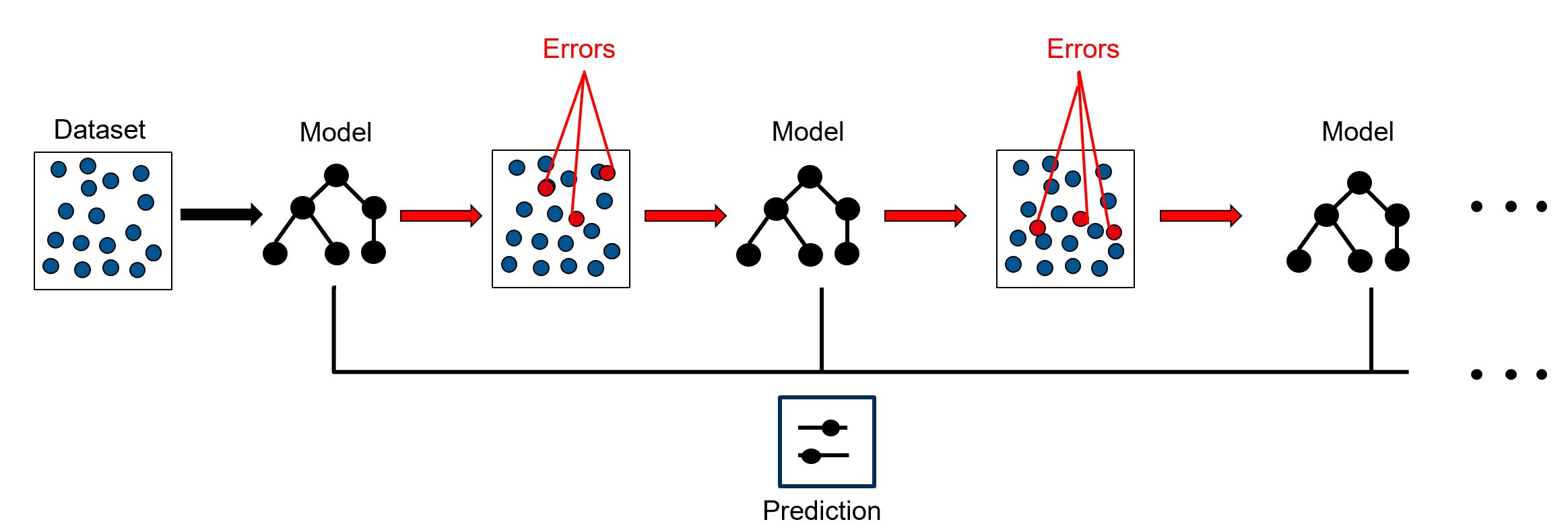
FIGURE 11.1: Simplified visualization of a gradient boosting machine. One trains a model based on the data. Then you fit a model to the resulting residuals. The result is then used to create a new model. This process is repeated until the desired result is achieved.
The over- and underfitting behavior of gradient boosting machines can be controlled via several regularization hyperparameters. An overfitting model can be trained by setting e.g. a high max_depth, i.e. the depth of trees fitted in each iteration, or a low min_bucket, i.e a low minimum of samples that need to be present in each leaf in order to allow for further splitting. Vice-versa, an underfitting can be created by adjusting the hyper-parameters in the opposite direction. This results in a very flexible algorithm, that allows us to cover various situations between underfitting, good fit and overfitting.
11.3.2 Data sets used for calculations
As Mentioned above, we want to use to different data sets:
A self-created data set with pre-specified correlation structure.
A real data set to see if the observations made under "laboratory conditions" can also be observed in the real world.
Our self created data set looks as follows:
- Uncorrelated features which leads to a \(0\)/\(1\)-classification
- \(x1\), \(x2\), \(x3\) and \(x4\) normally distributed with zero mean and standard deviation of 1
- Target variable based on linear function with a bias.
- Same data set with 2 highly correlated features \(x1\) and \(x2\) (correlation of \(0.9\))
The second data set is the IBM Watson Analytics Lab data for employee attrition:
- Uncover factors that lead to employee attrition
Dataset contains 1470 rows
Used Features:- Overtime
- Job Satisfaction
- Years at Company
- Age
- Gender
- Business Travel
- Monthly Income
- Distance from home
- Work-Life-Balance
- Education
- Years in current role
With these data sets, several models are fitted in order to generate over- and underfitting. The results are listed in the following section
11.3.3 Results
In this section we want to give an overview of the results of the comparison between the calculation of permutation feature importance based on the test and the training data.
We will start with the uncorrelated self created data set. Then the correlated self created data set and in the end we will have a look at the IBM Watson Employee Attrition data set.
Self created Data Set without Correlation
First, we will have the two permutation feature importance plots for a well tuned gradient boosting machine. We have four features, created based on the following formula:
\(z = 1 + 2*x1 + 3*x2 + x3 + 4*x4\)
On the x-axis you can see the feature importance and on the y-axis the feature.

FIGURE 11.2: The used features are located on the x-axis. The corresponding permutation feature importance can be found on the y-axis. x4 ist the most important feature, followed by x2, x1 and x3

FIGURE 11.3: Again, x4 ist the most important feature, followed by x2, x1 and x3. The range of the PFI values differes from 1 - 4 and is therefore wider than the range regarding the test data
As you can see, both plots are quite similar. The order of test and training data is exactly the same. \(x4\) is the most important feature, followed by \(x2\) and \(x1\). The least important feature is \(x3\).
Furthermore, the range of the two plots is not the same - but comparable. The PFI-plot based on test data has a range from 1 to 2.4 and the PFI-plot based on training data from 1.1 to 4. This indicates still an overfit of the GBM.
Now, we used the same data set but an overfitting GBM. You can find the corresponding plots below:
## Warning in use.package("data.table"): data.table
## cannot be used without R package bit64 version 0.9.7 or
## higher. Please upgrade to take advangage of data.table
## speedups.

## Warning in use.package("data.table"): data.table
## cannot be used without R package bit64 version 0.9.7 or
## higher. Please upgrade to take advangage of data.table
## speedups.

## Warning in use.package("data.table"): data.table
## cannot be used without R package bit64 version 0.9.7 or
## higher. Please upgrade to take advangage of data.table
## speedups.

## Warning in use.package("data.table"): data.table
## cannot be used without R package bit64 version 0.9.7 or
## higher. Please upgrade to take advangage of data.table
## speedups.

## Warning in use.package("data.table"): data.table
## cannot be used without R package bit64 version 0.9.7 or
## higher. Please upgrade to take advangage of data.table
## speedups.

## Warning in use.package("data.table"): data.table
## cannot be used without R package bit64 version 0.9.7 or
## higher. Please upgrade to take advangage of data.table
## speedups.

## Warning in use.package("data.table"): data.table
## cannot be used without R package bit64 version 0.9.7 or
## higher. Please upgrade to take advangage of data.table
## speedups.

## Warning in use.package("data.table"): data.table
## cannot be used without R package bit64 version 0.9.7 or
## higher. Please upgrade to take advangage of data.table
## speedups.

## Warning in use.package("data.table"): data.table
## cannot be used without R package bit64 version 0.9.7 or
## higher. Please upgrade to take advangage of data.table
## speedups.

## Warning in use.package("data.table"): data.table
## cannot be used without R package bit64 version 0.9.7 or
## higher. Please upgrade to take advangage of data.table
## speedups.

## Warning in use.package("data.table"): data.table
## cannot be used without R package bit64 version 0.9.7 or
## higher. Please upgrade to take advangage of data.table
## speedups.

## Warning in use.package("data.table"): data.table
## cannot be used without R package bit64 version 0.9.7 or
## higher. Please upgrade to take advangage of data.table
## speedups.

## Warning in use.package("data.table"): data.table
## cannot be used without R package bit64 version 0.9.7 or
## higher. Please upgrade to take advangage of data.table
## speedups.

## Warning in use.package("data.table"): data.table
## cannot be used without R package bit64 version 0.9.7 or
## higher. Please upgrade to take advangage of data.table
## speedups.

## Warning in use.package("data.table"): data.table
## cannot be used without R package bit64 version 0.9.7 or
## higher. Please upgrade to take advangage of data.table
## speedups.

## Warning in use.package("data.table"): data.table
## cannot be used without R package bit64 version 0.9.7 or
## higher. Please upgrade to take advangage of data.table
## speedups.

## Warning in use.package("data.table"): data.table
## cannot be used without R package bit64 version 0.9.7 or
## higher. Please upgrade to take advangage of data.table
## speedups.

## Warning in use.package("data.table"): data.table
## cannot be used without R package bit64 version 0.9.7 or
## higher. Please upgrade to take advangage of data.table
## speedups.

## Warning in use.package("data.table"): data.table
## cannot be used without R package bit64 version 0.9.7 or
## higher. Please upgrade to take advangage of data.table
## speedups.

## Warning in use.package("data.table"): data.table
## cannot be used without R package bit64 version 0.9.7 or
## higher. Please upgrade to take advangage of data.table
## speedups.

## Warning in use.package("data.table"): data.table
## cannot be used without R package bit64 version 0.9.7 or
## higher. Please upgrade to take advangage of data.table
## speedups.

## Warning in use.package("data.table"): data.table
## cannot be used without R package bit64 version 0.9.7 or
## higher. Please upgrade to take advangage of data.table
## speedups.
FIGURE 11.4: For an overfitting GBM the order for test data is the same as seen before in the well fitted case. The range of the test data is quite the same as before.
## Warning in use.package("data.table"): data.table
## cannot be used without R package bit64 version 0.9.7 or
## higher. Please upgrade to take advangage of data.table
## speedups.

## Warning in use.package("data.table"): data.table
## cannot be used without R package bit64 version 0.9.7 or
## higher. Please upgrade to take advangage of data.table
## speedups.

## Warning in use.package("data.table"): data.table
## cannot be used without R package bit64 version 0.9.7 or
## higher. Please upgrade to take advangage of data.table
## speedups.

## Warning in use.package("data.table"): data.table
## cannot be used without R package bit64 version 0.9.7 or
## higher. Please upgrade to take advangage of data.table
## speedups.

## Warning in use.package("data.table"): data.table
## cannot be used without R package bit64 version 0.9.7 or
## higher. Please upgrade to take advangage of data.table
## speedups.

## Warning in use.package("data.table"): data.table
## cannot be used without R package bit64 version 0.9.7 or
## higher. Please upgrade to take advangage of data.table
## speedups.

## Warning in use.package("data.table"): data.table
## cannot be used without R package bit64 version 0.9.7 or
## higher. Please upgrade to take advangage of data.table
## speedups.

## Warning in use.package("data.table"): data.table
## cannot be used without R package bit64 version 0.9.7 or
## higher. Please upgrade to take advangage of data.table
## speedups.

## Warning in use.package("data.table"): data.table
## cannot be used without R package bit64 version 0.9.7 or
## higher. Please upgrade to take advangage of data.table
## speedups.

## Warning in use.package("data.table"): data.table
## cannot be used without R package bit64 version 0.9.7 or
## higher. Please upgrade to take advangage of data.table
## speedups.

## Warning in use.package("data.table"): data.table
## cannot be used without R package bit64 version 0.9.7 or
## higher. Please upgrade to take advangage of data.table
## speedups.

## Warning in use.package("data.table"): data.table
## cannot be used without R package bit64 version 0.9.7 or
## higher. Please upgrade to take advangage of data.table
## speedups.

## Warning in use.package("data.table"): data.table
## cannot be used without R package bit64 version 0.9.7 or
## higher. Please upgrade to take advangage of data.table
## speedups.

## Warning in use.package("data.table"): data.table
## cannot be used without R package bit64 version 0.9.7 or
## higher. Please upgrade to take advangage of data.table
## speedups.

## Warning in use.package("data.table"): data.table
## cannot be used without R package bit64 version 0.9.7 or
## higher. Please upgrade to take advangage of data.table
## speedups.

## Warning in use.package("data.table"): data.table
## cannot be used without R package bit64 version 0.9.7 or
## higher. Please upgrade to take advangage of data.table
## speedups.

## Warning in use.package("data.table"): data.table
## cannot be used without R package bit64 version 0.9.7 or
## higher. Please upgrade to take advangage of data.table
## speedups.

## Warning in use.package("data.table"): data.table
## cannot be used without R package bit64 version 0.9.7 or
## higher. Please upgrade to take advangage of data.table
## speedups.

## Warning in use.package("data.table"): data.table
## cannot be used without R package bit64 version 0.9.7 or
## higher. Please upgrade to take advangage of data.table
## speedups.

## Warning in use.package("data.table"): data.table
## cannot be used without R package bit64 version 0.9.7 or
## higher. Please upgrade to take advangage of data.table
## speedups.

## Warning in use.package("data.table"): data.table
## cannot be used without R package bit64 version 0.9.7 or
## higher. Please upgrade to take advangage of data.table
## speedups.

## Warning in use.package("data.table"): data.table
## cannot be used without R package bit64 version 0.9.7 or
## higher. Please upgrade to take advangage of data.table
## speedups.
FIGURE 11.5: For an overfitting GBM the order for training data is the same as seen before in the well fitted case. In contrast to quite similar values of PFI, the range now differs a lot between test and training data and between training data in the well- and overfitting case
At first sight these two plots look very similar to the first two. The order of the features has remained the same and the relative distances to each other are also very similar. It is also noticeable that the plot regarding the test data has hardly changed - whereas the range of the permutation feature importance based on training data has become much wider. This is a typical behavior of overfitting in terms of feature importance, since the models learns to use a variable "better" than it actually is.
The last 2 plots for the uncorrelated data set are the ones of an underfitting GBM:
## Warning in use.package("data.table"): data.table
## cannot be used without R package bit64 version 0.9.7 or
## higher. Please upgrade to take advangage of data.table
## speedups.

## Warning in use.package("data.table"): data.table
## cannot be used without R package bit64 version 0.9.7 or
## higher. Please upgrade to take advangage of data.table
## speedups.

## Warning in use.package("data.table"): data.table
## cannot be used without R package bit64 version 0.9.7 or
## higher. Please upgrade to take advangage of data.table
## speedups.

## Warning in use.package("data.table"): data.table
## cannot be used without R package bit64 version 0.9.7 or
## higher. Please upgrade to take advangage of data.table
## speedups.

## Warning in use.package("data.table"): data.table
## cannot be used without R package bit64 version 0.9.7 or
## higher. Please upgrade to take advangage of data.table
## speedups.

## Warning in use.package("data.table"): data.table
## cannot be used without R package bit64 version 0.9.7 or
## higher. Please upgrade to take advangage of data.table
## speedups.

## Warning in use.package("data.table"): data.table
## cannot be used without R package bit64 version 0.9.7 or
## higher. Please upgrade to take advangage of data.table
## speedups.

## Warning in use.package("data.table"): data.table
## cannot be used without R package bit64 version 0.9.7 or
## higher. Please upgrade to take advangage of data.table
## speedups.

## Warning in use.package("data.table"): data.table
## cannot be used without R package bit64 version 0.9.7 or
## higher. Please upgrade to take advangage of data.table
## speedups.

## Warning in use.package("data.table"): data.table
## cannot be used without R package bit64 version 0.9.7 or
## higher. Please upgrade to take advangage of data.table
## speedups.

## Warning in use.package("data.table"): data.table
## cannot be used without R package bit64 version 0.9.7 or
## higher. Please upgrade to take advangage of data.table
## speedups.

## Warning in use.package("data.table"): data.table
## cannot be used without R package bit64 version 0.9.7 or
## higher. Please upgrade to take advangage of data.table
## speedups.

## Warning in use.package("data.table"): data.table
## cannot be used without R package bit64 version 0.9.7 or
## higher. Please upgrade to take advangage of data.table
## speedups.

## Warning in use.package("data.table"): data.table
## cannot be used without R package bit64 version 0.9.7 or
## higher. Please upgrade to take advangage of data.table
## speedups.

## Warning in use.package("data.table"): data.table
## cannot be used without R package bit64 version 0.9.7 or
## higher. Please upgrade to take advangage of data.table
## speedups.

## Warning in use.package("data.table"): data.table
## cannot be used without R package bit64 version 0.9.7 or
## higher. Please upgrade to take advangage of data.table
## speedups.

## Warning in use.package("data.table"): data.table
## cannot be used without R package bit64 version 0.9.7 or
## higher. Please upgrade to take advangage of data.table
## speedups.

## Warning in use.package("data.table"): data.table
## cannot be used without R package bit64 version 0.9.7 or
## higher. Please upgrade to take advangage of data.table
## speedups.

## Warning in use.package("data.table"): data.table
## cannot be used without R package bit64 version 0.9.7 or
## higher. Please upgrade to take advangage of data.table
## speedups.

## Warning in use.package("data.table"): data.table
## cannot be used without R package bit64 version 0.9.7 or
## higher. Please upgrade to take advangage of data.table
## speedups.

## Warning in use.package("data.table"): data.table
## cannot be used without R package bit64 version 0.9.7 or
## higher. Please upgrade to take advangage of data.table
## speedups.

## Warning in use.package("data.table"): data.table
## cannot be used without R package bit64 version 0.9.7 or
## higher. Please upgrade to take advangage of data.table
## speedups.
FIGURE 11.6: PFI plot of an underfitting GBM based on test data. The importance is now reduced with highest value at around 1.6 in contrast to 2.4 before. Furthermore, x1 is the least important feature now.
## Warning in use.package("data.table"): data.table
## cannot be used without R package bit64 version 0.9.7 or
## higher. Please upgrade to take advangage of data.table
## speedups.

## Warning in use.package("data.table"): data.table
## cannot be used without R package bit64 version 0.9.7 or
## higher. Please upgrade to take advangage of data.table
## speedups.

## Warning in use.package("data.table"): data.table
## cannot be used without R package bit64 version 0.9.7 or
## higher. Please upgrade to take advangage of data.table
## speedups.

## Warning in use.package("data.table"): data.table
## cannot be used without R package bit64 version 0.9.7 or
## higher. Please upgrade to take advangage of data.table
## speedups.

## Warning in use.package("data.table"): data.table
## cannot be used without R package bit64 version 0.9.7 or
## higher. Please upgrade to take advangage of data.table
## speedups.

## Warning in use.package("data.table"): data.table
## cannot be used without R package bit64 version 0.9.7 or
## higher. Please upgrade to take advangage of data.table
## speedups.

## Warning in use.package("data.table"): data.table
## cannot be used without R package bit64 version 0.9.7 or
## higher. Please upgrade to take advangage of data.table
## speedups.

## Warning in use.package("data.table"): data.table
## cannot be used without R package bit64 version 0.9.7 or
## higher. Please upgrade to take advangage of data.table
## speedups.

## Warning in use.package("data.table"): data.table
## cannot be used without R package bit64 version 0.9.7 or
## higher. Please upgrade to take advangage of data.table
## speedups.

## Warning in use.package("data.table"): data.table
## cannot be used without R package bit64 version 0.9.7 or
## higher. Please upgrade to take advangage of data.table
## speedups.

## Warning in use.package("data.table"): data.table
## cannot be used without R package bit64 version 0.9.7 or
## higher. Please upgrade to take advangage of data.table
## speedups.

## Warning in use.package("data.table"): data.table
## cannot be used without R package bit64 version 0.9.7 or
## higher. Please upgrade to take advangage of data.table
## speedups.

## Warning in use.package("data.table"): data.table
## cannot be used without R package bit64 version 0.9.7 or
## higher. Please upgrade to take advangage of data.table
## speedups.

## Warning in use.package("data.table"): data.table
## cannot be used without R package bit64 version 0.9.7 or
## higher. Please upgrade to take advangage of data.table
## speedups.

## Warning in use.package("data.table"): data.table
## cannot be used without R package bit64 version 0.9.7 or
## higher. Please upgrade to take advangage of data.table
## speedups.

## Warning in use.package("data.table"): data.table
## cannot be used without R package bit64 version 0.9.7 or
## higher. Please upgrade to take advangage of data.table
## speedups.

## Warning in use.package("data.table"): data.table
## cannot be used without R package bit64 version 0.9.7 or
## higher. Please upgrade to take advangage of data.table
## speedups.

## Warning in use.package("data.table"): data.table
## cannot be used without R package bit64 version 0.9.7 or
## higher. Please upgrade to take advangage of data.table
## speedups.

## Warning in use.package("data.table"): data.table
## cannot be used without R package bit64 version 0.9.7 or
## higher. Please upgrade to take advangage of data.table
## speedups.

## Warning in use.package("data.table"): data.table
## cannot be used without R package bit64 version 0.9.7 or
## higher. Please upgrade to take advangage of data.table
## speedups.

## Warning in use.package("data.table"): data.table
## cannot be used without R package bit64 version 0.9.7 or
## higher. Please upgrade to take advangage of data.table
## speedups.

## Warning in use.package("data.table"): data.table
## cannot be used without R package bit64 version 0.9.7 or
## higher. Please upgrade to take advangage of data.table
## speedups.
FIGURE 11.7: Overall, the importance is reduced. X3 is still the least important one. All PFI values are lower than before
With the plots for an underfitting GBM it is noticeable that the range is almost the same - but at a low level (from 1-1.8 or 1-1.6). Most noticeable, however, is that the order has changed. Based on the test data, \(x1\) is now the least important variable. Overall, the feature importance decreases - and therefore a change in the positions becomes more probable.
Self created Data Set without Correlation
Now, we used the same data set but included 2 highly correlated features. The correlation between \(x1\) and \(x2\) is set to 0.9.
In the first plot the results for a well tuned GBM are compared for test and training data. The noteworthy areas are highlighted in red.
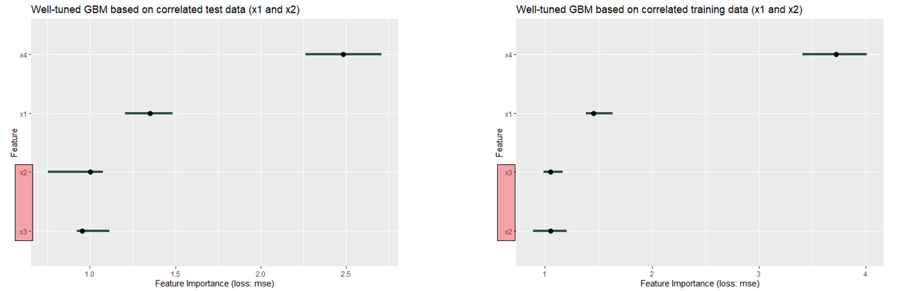
FIGURE 11.8: For the well fitted GBM at the correlated self created data set, the order differs. For the test data x4 ist the most important feature followed by x1, x2 and x3 whereas for the training data x2 and x3 changed places
The order of the features has changed - but in the area of features that are close to 1 (i.e. unimportant features).
In the next plot, we want to compare test and training data permutation feature importance of an overfitting GBM:
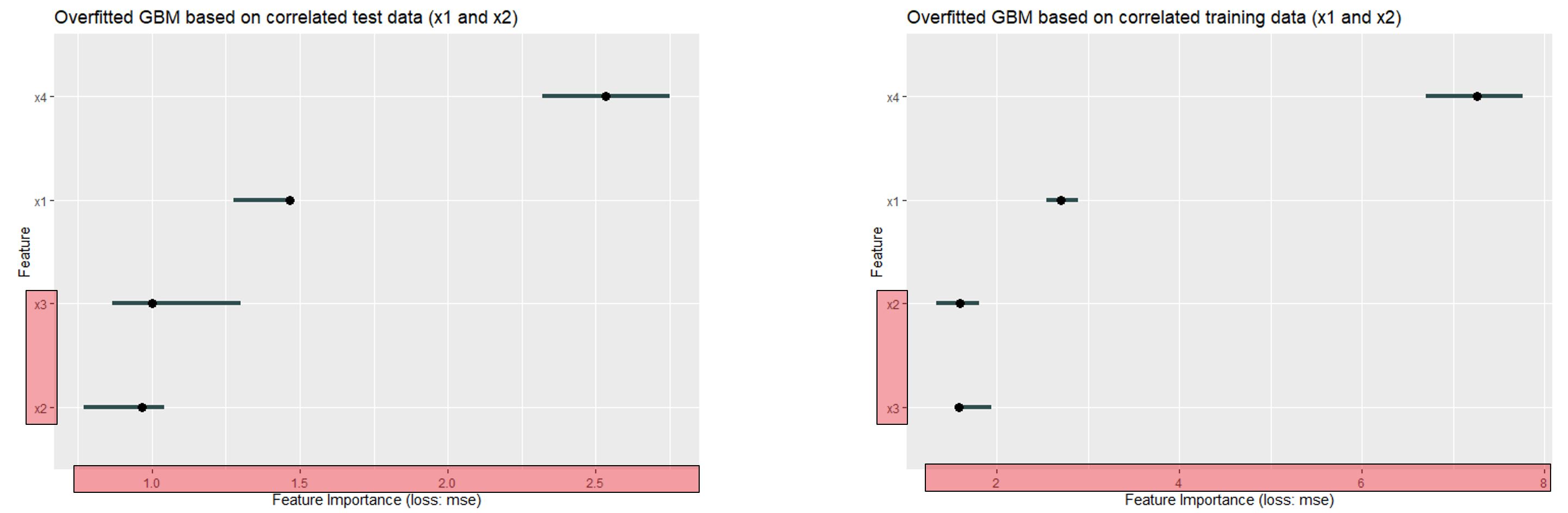
FIGURE 11.9: x4 is the most important feature in both plots. Followed by x1, x3 and x2 in descending order for the test data - and again x2 and x3 changed places for the training data. It has to be stated, that the range for training data is much wider.
The range for the training data set is much wider again - similar to the range for the uncorrelated data. In addition it is noticeable that the order has changed in the lower range - which is again due to the fact that the less important features are close to 1 (i.e. have no influence on the MSE).
The last plot for correlated data used an underfitting GBM: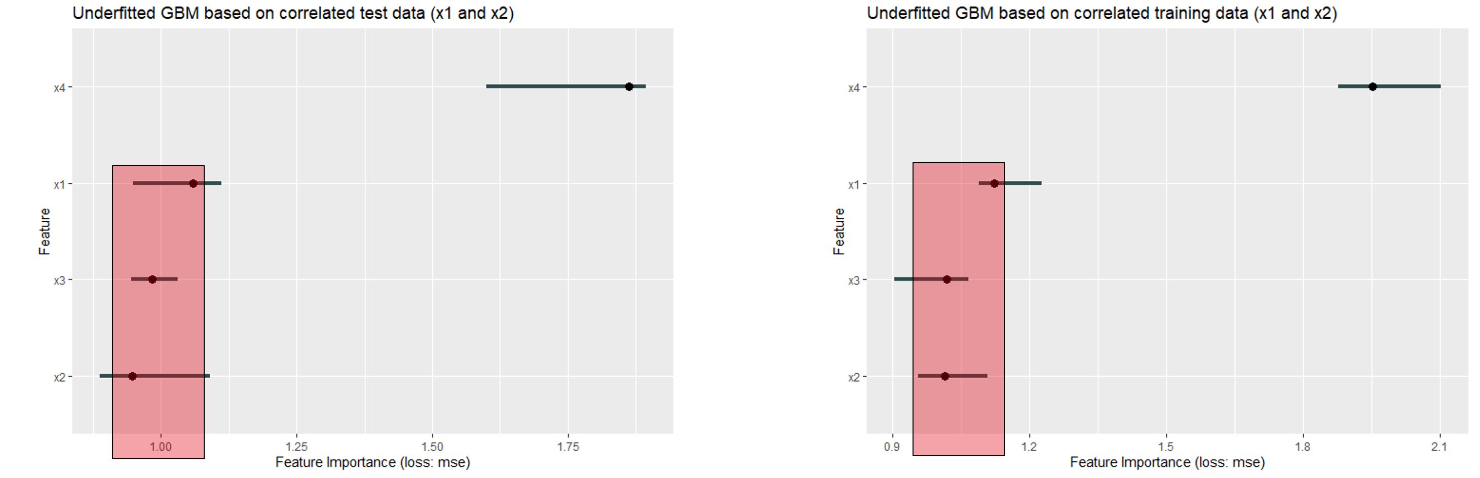
FIGURE 11.10: x4 is the most important feature in both plots. Followed by x1, x3 and x2 in descending order. Except x4 all permutation feature importance values are close to 1
It can be said that the order has remained the same - but \(x1\) \(x2\) and \(x3\) are very close to a feature importance of 1 (which means: no influence on the MSE). Furthermore, the range is very comparable.
IBM Watson Data of Employee Attrition
Finally, we will take a look at how test and training data behave outside laboratory conditions with real data. Here we looked at which variables contribute to an employee leaving the company.
Again, we compared the permutation feature importance of test and training data set.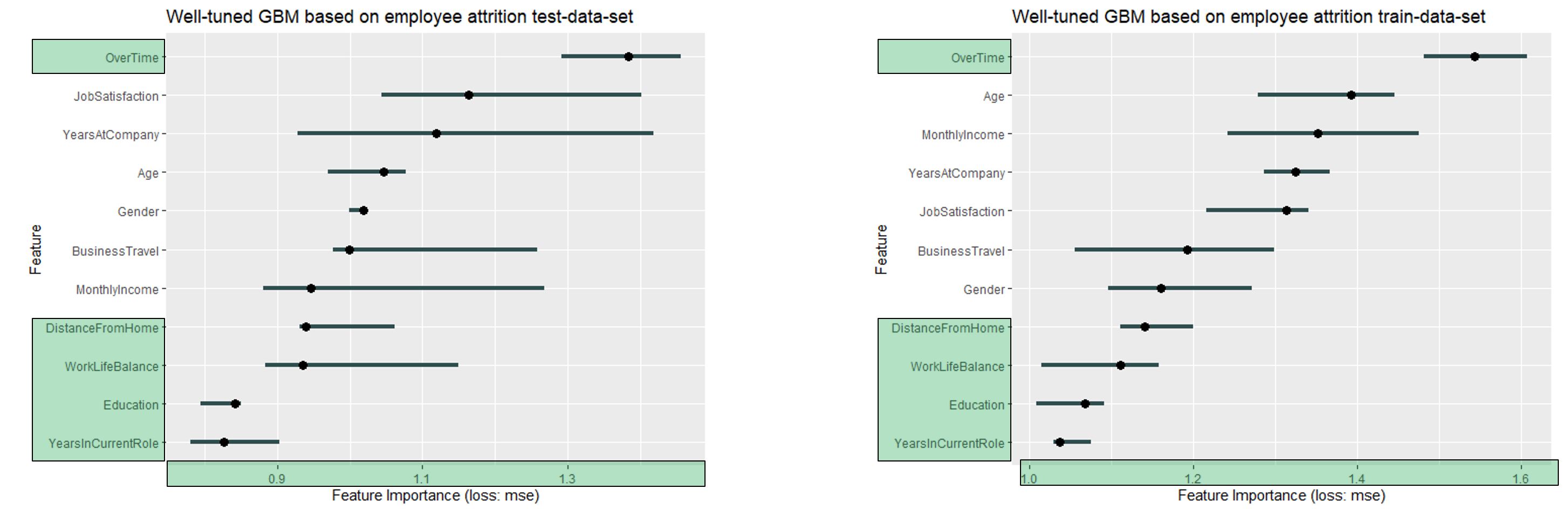
FIGURE 11.11: For both data sets Overtime is the most important feature. Furthermore, the 4 least important variables are the same - and in the same order (Dist from home, WorkLifeBalance, Education and YearsInCurrentRole)
The noticeable features are highlighted in green. As with the previous well fitted GBM, the range is very comparable - the order has also remained the same, at least in parts. (Overtime is the most important variable in both cases)
Also here we want to have a look at the behavior at over- and underfitting.
We start again with the plots for overfitting:
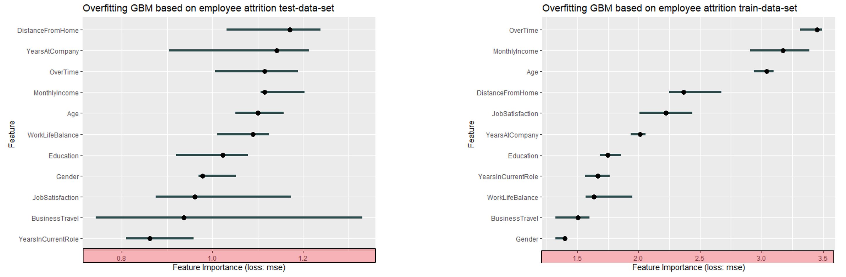
FIGURE 11.12: For the test data based on an overfitting GBM, DistanceFromHome is the most important variable. For the training data it is only the fourth most important one, wheras Overtime is most important. It can be stated that the order changed a lot
There's really a lot going on here. Both the range (as always with overfitting) and the order change a lot. The results are not comparable in any way.
Last but not least we will have a look at the underfitting GBM for the IBM Watson data set:
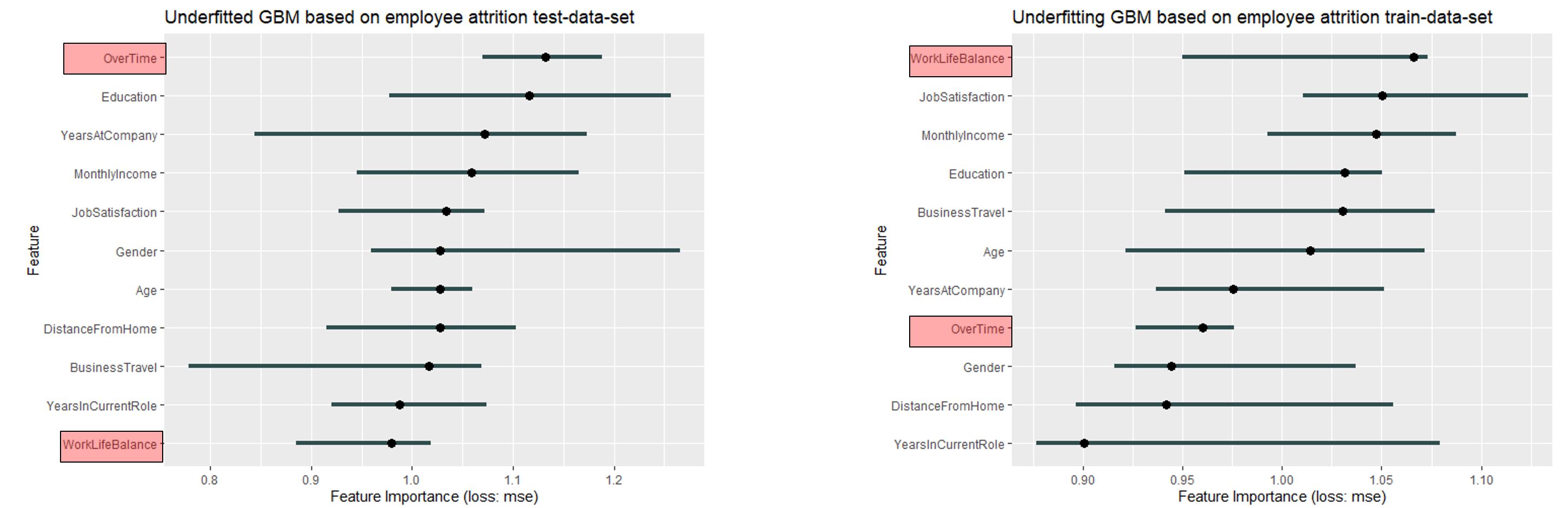
FIGURE 11.13: In this Figure it is quite interesting that the order changed completly. Overtime is the most important variable based on the test data and is only at place number 8 for the training data. Even more extreme is the case with WorkLifeBalance
The range is comparable - but very small (0.9 - 1.2). Again underfitting has a reducing effect on the feature importance. In addition, the order has changed extremely (work life balance has changed from the least important variable at the test data to the most important variable at the training data).
11.3.4 Interpretation of the results
At the end of this sub-chapter we want to answer the question how the permutation feature importance behaves with regard to over- and underfitting. First, it can be said that in the case of a well fit GBM there are only slight differences in feature importance. The results on test and training data are in any case comparable. But now we come to the problems regarding the meaningfulness of feature importance:
Problems with overfitting:
- Overfitting results in a very strong effect on the MSE only on the training data
- Furthermore, the order differs a lot
Problems with underfitting:
- The effect on the MSE is low - the results a consistently lower
- As in the overfitting case the order differs a lot
Over- and underfitting has definitely an impact on feature importance
Our third question was, if correlation does effect the decision whether to use test or training data for calculating the permutation feature importance:
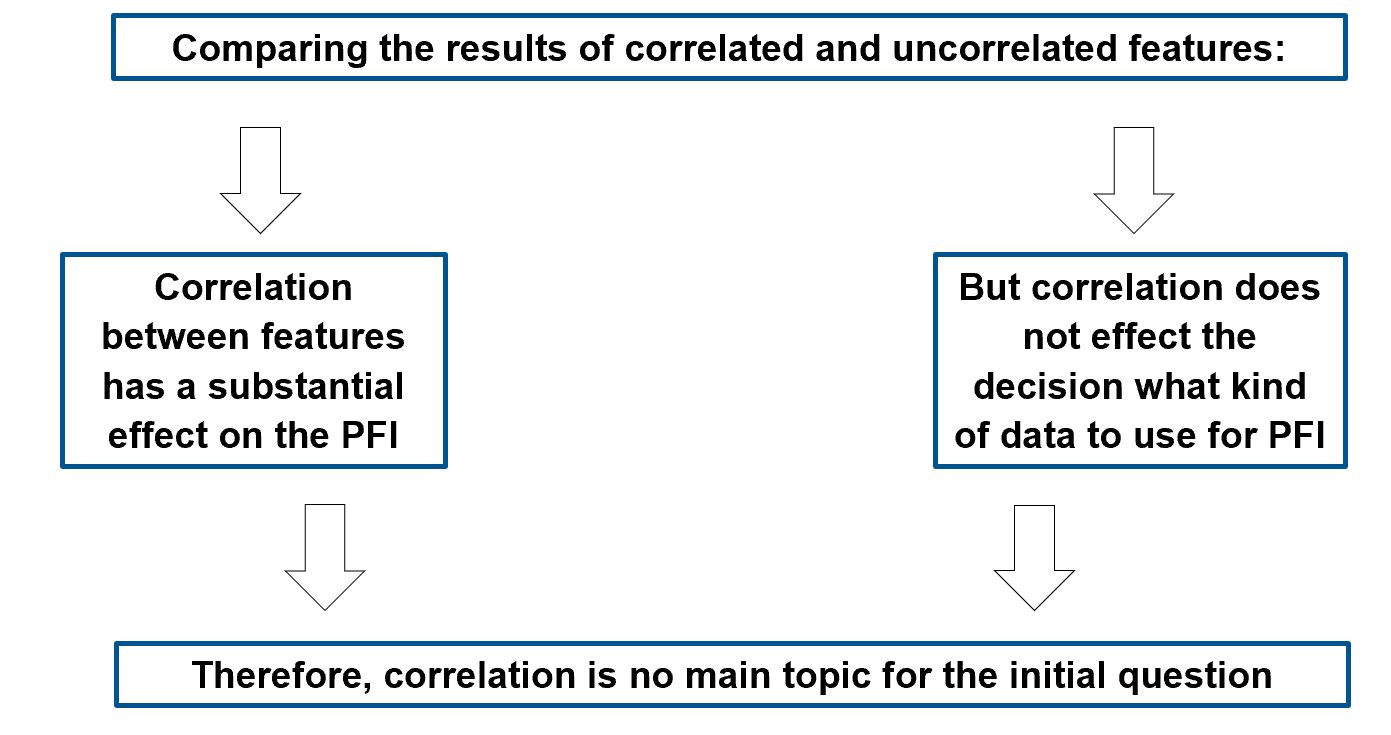
FIGURE 11.14: Visualisation of the impact of correlation on the feature importance. As you have seen above, correlation is a problem regarding permutation feature importance but does not effect the decision regarding test vs. training data
11.4 Summary
The Question what data set you use for calculation of the permutation feature importance still depends on what you are interested in:
- Contribution to the performance on unknown data?
or
- How much the model relies for prediction?
It was shown that PFI reacts strongly to over- and underfitting:
- PFI on both can be a proxy identifying over- or underfitting
Correlated features have a big influence on the results of feature importance, but not on the question whether to use test or training data - therefore they are negligible in this question. Nevertheless, correlations have been shown to lead to major feature importance problems, as discussed in previous chapters.
Basically it can be said that it has been shown that the model behavior (overfitting or underfitting) greatly distorts the interpretation of the feature importance. Therefore it is important to set up your model well, because it was shown that the differences for a well calibrated model are only small and the question of choice doesn't play a big role anymore.
References
Molnar, Christoph. 2019. Interpretable Machine Learning: A Guide for Making Black Box Models Explainable.