Chapter 7 ALE Intervals, Piece-Wise Constant Models and Categorical Features

Author: Nikolas Fritz

Supervisor: Christian Scholbeck

As mentioned in the former section the choice of intervals and starting value \(z_{0,j}\) have both a certain influence on the estimated ALE - curve. While the main influence of \(z_{0,j}\) is canceled out by centering the ALE, the choice of intervals stays crucial. Therefore the next section is dedicated to this topic.

7.1 How to choose the number and/or length of the intervals

Before investigating the choice of intervals one should be clear about how far they influence the estimation. On the one hand for a given interval the ALE estimation will be linear due to the expected constant effect within this interval. Remember that within each interval the local effect within this interval was calculated by the mean total difference of the prediction when shifting the variable of interest from the lower interval boundary to the upper one. This leads by definition to a constant effect within this interval that results in a linear function when integrating over the interval.
It seems obvious that the ALE estimation (within a grid interval) can only be as good as a linear approximation for the "real" and usually unknown prediction function can be. Therefore it is crucial for a good estimation to have small enough intervals especially in regions where the prediction function is shaky or far from linear (i.e high second derivatives) with respect to the feature of interest. On the other hand, to get stable estimations for a grid interval it is important to have a sufficiently high number of data points within the interval. This means that the intervals shouldn't become too small so that they would contain only a few data points. Note that this is only true if the other features have an influence on the local effect of the prediction function. If they don't, any data point within the grid interval would lead to the same predictions at the interval boundaries. That's why there is a natural trade-off between a small interval width and the number of the contained data points.

7.1.1 State of the art

So the question is how to optimally choose the grid intervals. Should they all be of the same width containing a different number of data points? Should they all contain the same or at least a similar number of data points, accepting different interval sizes. Or could there even be a better solution in between the two concepts?
Within the iml-package which is one of two implementations of ALE - plots the chosen method is the second one. The quantiles of the distribution of the feature are used as the grid that defines the intervals. That means the length of the intervals depends on the chosen grid size and the given feature distribution.

In the following section, some examples with artificial data sets are provided, that should help to get a better feeling for the different deterministic factors that influence the goodness of the ALE estimation. Within the whole chapter, the ALE estimation is conducted via the iml-package implementation.

7.1.2 ALE Approximations

In the following section, we only consider two-dimensional data sets, of continuous features \(x_1\) and \(x_2\) with a certain correlation. Furthermore, we use some exemplary prediction functions which are differentiable such that we can calculate the theoretical ALE (see section 5.2) and use it to evaluate the goodness of the estimated ALE - curve. As we want to isolate some of the above mentioned influential factors, we start with some easy examples adding step by step more complexity to the problem.

7.1.3 Example 1: additive feature effects

In the first example we assume a uniform distribution for the feature \(x_1\) on the interval \([0, 10]\), i.e. \(X_1 \sim U(0,10)\). Furthermore we assume the conditional distribution of the feature \(x_2\) given \(x_1\) to be also uniform on the interval \([x_1 - 3,~x_1 + 3 ]\), i.e. \(X_2 \vert X_1 = x_1 \sim U(x_1 - 3,~x_1 + 3 )\). Sampling 100 data points from this distribution yields the first dataset (see Figure 7.1) .

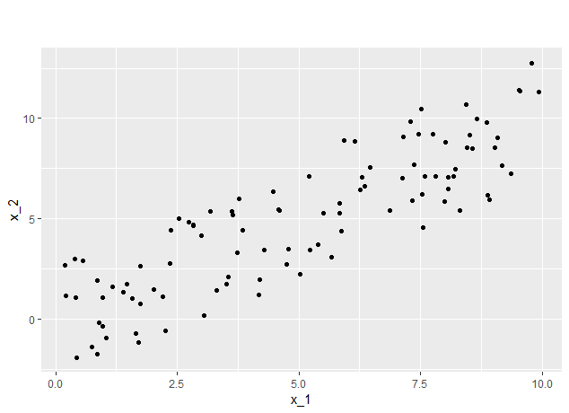
FIGURE 7.1: The correlation is clearly recognizable.

Why we only made assumptions about the conditional distributon of \(X_2\) and not on the joint distribution of \((X_1,X_2)\) gets clearer once we take a look on the calculation of the theoratical ALE. Therefore we first asume the prediction function \(\hat{f}_1 (x_1, x_2) = (x_1-4)(x_1-5)(x_1-6) + x_2^3\). Due to the special structure of \(f_1\) the partial derivative with respect to \(x_1\) is a polynomial of degree 2 which doesn't depend on \(x_2\), concretley \(\hat{f}^1(x_1,x_2) = 3x_1^2 -30x_1 +74\) (Remember the unusual notation for the j-th partial derivative as \(f^{j}\)). Now we can calculate the theoretical (uncentered) ALE:

\[(1)~~~~\widetilde{ALE}_{\hat{f},1}(x) = \int_{z_{0,1}}^x E_{X_2\vert X_1= Z_1}[\hat{f}^1(x_1,x_2)]~dz~~~=\] \[(2)~~~~ \int_{z_{0,1}}^x \int p_{X_2\vert X_1 = z }(x_2)\hat{f}^1(z,x_2)~dx_2~dz~~~=\] \[(3)~~~~ \int_{z_{0,1}}^x \hat{f}^1(z,x_2)\int p_{X_2\vert X_1=z}(x_2)~dx_2~dz~~~=\]

\[(4)~~~~ \int_{z_{0,1}}^x \hat{f}^1(z,x_2)~dz~~~=\] \[(5)~~~~ \int_{z_{0,1}}^x 3z^2 -30z +74~dz~~~=\] \[(6)~~~~ [z^3 -15z^2 +74z + c]_{z_{0,1}}^x~~~=\]

\[(7)~~~~ x^3 -15x^2 +74x - z_{0,1} ^ 3 + 15 z_{0,1}^2 - 74z_{0,1}~~~\] Here \(p_{X_2\vert X_1=z}(x_2)\) notates the conditional density of \(X_2\vert X_1\) for \(x_1 = z\).
Step (3) makes use of the fact that \(\hat{f}^1(x_1,x_2)\) doesn't depend on \(x_2\) and in step (4) the integral over the density gives 1. To get the centered ALE we have to calculate:

\[(8)~~~~ALE_{\hat{f},1}(x) = \widetilde{ALE}_{\hat{f},1}(x) - E[\widetilde{ALE}_{\hat{f},1}(X_1)] ~~~=\]

\[(9)~~~~ x^3 - 15x^2 +74x - z_{0,1} ^ 3 + 15 z_{0,1}^2 - 74z_{0,1} ~- \]

\[ E[X_1^3 -15X_1^2 +74X_1 - z_{0,1} ^ 3 + 15 z_{0,1}^2 - 74z_{0,1}] ~~~=\]

\[(10)~~~~ x^3 -15x^2 +74x - E[X_1^3 -15X_1^2 +74X_1] ~~~=\]

\[(11)~~~~ x^3 -15x^2 +74x - E[X_1^3] +15E[X_1^2] -74E[X_1] ~~~=\]

\[(12)~~~~ x^3 -15x^2 +74x - 250 +15 \frac{100}{3}) - 74* 5 ~~~=\]

\[(13)~~~~ x^3 -15x^2 +74x - 120~~~.\]

In Step (12) the formula for the kth - moment of the uniform distribution which is given by \(m_k = \frac{1}{k+1}\sum_{i=0}^k a^i b^{k-i}\) was used. Knowing the theoretical ALE-curve we can have a look at the behavior of the estimated ALE for different grid sizes. Figure 7.2 shows the theoretical ALE and the estimations for grid sizes 2, 3, 5, and 10.

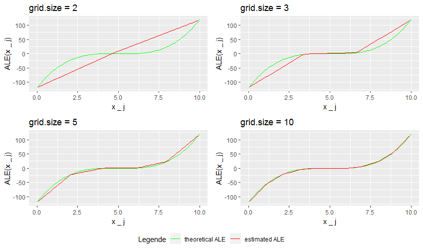
FIGURE 7.2: Theoretical vs estimated ALE

While the estimated ALE with grid size 2 only shows a linear effect over the whole data range, the estimated ALE with grid size 3 already gives a good approximation to the theoretical ALE in the second interval, where the theoretical ALE has a low curvature. With grid size 5 only the outer intervals show clearly recognizable deviations to the theoretical ALE and with grid size 10 the approximation looks quite reasonable. As the partial derivative of the prediction function was independent of \(x_2\), there was no risk of getting bad estimations due to too few data points within an interval. That's why we take a look at a second example.

7.1.4 Example 2: multiplicative feature effects

Now we asume the prediction function \(\hat{f}_2 (x_1, x_2) = (x_1-4)(x_1-5)(x_1-6)x_2^3\). In this case the partial derivative with respect to \(x_1\) is a polynomial of degree 2 which clearly depends on \(x_2\), concretley \(\hat{f}^1(x_1,x_2) = (3x_1^2 -30x_1 +74)x_2^3\). The new structure of the partial derivative yields a new calculation for the theoretical uncentered ALE:

\[(1)~~~~\widetilde{ALE}_{\hat{f},1}(x) = \int_{z_{0,1}}^x E_{X_2\vert X_1= Z_1}[\hat{f}^1(x_1,x_2)]~dz~~~=\]

\[(2)~~~~ \int_{z_{0,1}}^x \int p_{X_2\vert X_1=z}(x_2)\hat{f}^1(z,x_2)~dx_2~dz~~~=\] \[(3)~~~~ \int_{z_{0,1}}^x \int p_{X_2\vert X_1=z}(x_2)(3z^2 -30z +74)x_2^3~dx_2~dz~~~=\] \[(4)~~~~ \int_{z_{0,1}}^x (3z^2 -30z +74)\int p_{X_2\vert X_1=z}(x_2)x_2^3~dx_2~dz~~~=\] \[(5)~~~~ \int_{z_{0,1}}^x (3z^2 -30z +74)~E_{X_2\vert X_1 = z}[X_2^3]~dz~~~=\]

\[(6)~~~~ \int_{z_{0,1}}^x (3z^2 -30z +74)(\frac{1}{4}\sum_{i=0}^{k=3}(z-3)^i(z+3)^{k-i})~dz~~~=\] \[(7)~~~~ \int_{z_{0,1}}^x (3z^2 -30z +74)(z^3 + 9z)~dz~~~=\] \[(8)~~~~ \int_{z_{0,1}}^x 3 z^5 - 30 z^4 + 101 z^3 - 270 z^2 + 666 z ~dz~~~=\]

\[(9)~~~~ [ \frac{3}{6} z^6 - \frac{30}{5}z^5 + \frac{101}{4}z^4 - 90 z^3 + 333 z^2]_{z_{0,1}}^x~~~\] Centering yields

\[(10)~~~~ALE_{\hat{f},1}(x) = \frac{3}{6} x^6 - \frac{30}{5}x^5 + \frac{101}{4}x^4 - 90 x^3 + 333 x^2 - \]

\[E[ \frac{3}{6} X_1^6 - \frac{30}{5}X_1^5 + \frac{101}{4}X_1^4 - 90 X_1^3 + 333 X_1^2] ~~~\] Again using the formula for the moments of a uniform distribution we finally obtain

\[(11)~~~~ALE_{\hat{f},1}(x) = \frac{3}{6} x^6 - \frac{30}{5}x^5 + \frac{101}{4}x^4 - 90 x^3 + 333 x^2 - \]

\[(\frac{3}{6}\frac{10^6}{7}-\frac{30}{5}\frac{10^5}{6} +\frac{101}{4}\frac{10^4}{5}-90\frac{10^3}{4}+333\frac{10^2}{3}) ~~~=\]

\[(12)~~~~ALE_{\hat{f},1}(x) = \frac{3}{6} x^6 - \frac{30}{5}x^5 + \frac{101}{4}x^4 - 90 x^3 + 333 x^2 - 10528.57~~~.\] Figure 7.3 shows the behavior of the ALE with different grid sizes in this setting.

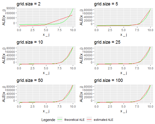
FIGURE 7.3: Theoretical vs estimated ALE for different grid sizes

While for grid size 5 and bigger the approximations for the region 0 to 7.5 seem quite reasonable it looks like for the region 7.5 to 10 the approximation is best for grid size 10 and gets worse with higher grid sizes. Zooming in for grid sizes 10 and 25 reveals this effect more clearly (Figure 7.4).

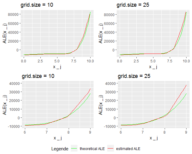
FIGURE 7.4: ALE-plots for grid sizes 10 and 25 (zoomed in)

Where does this come from? The structure of the prediction function leads to an increasing effect of \(x_2\) on the total differences calculated for the series of intervals. Due to insufficient many datapoints within the intervals, there is a high probability of under or overestimating this effect. With grid size 25 only 4 data points are used for the estimation. Obviously, it's quite probable that the \(x_2\) values of those data points are clearly above average in some intervals. If that happens for high \(x_1\) - which implies due to the correlation structure high \(x_2\) - the total difference will be clearly overestimated as the delta in \(x_1\) is multiplied by the average \(x_2^3\). As the effect on the intervals is accumulated, the error persists for the whole ALE-curve from that point on.

To get a deeper insight into this dynamic, for the given context ALE - curves for 50 sampled datasets were estimated with grid sizes 10, 25, and 50. For each grid size at each value of \(x_1\) the minimal and the maximal ALE estimation was taken as the boundary of the range of estimations. Figure 7.5 shows this range exemplarily for gride size 10.

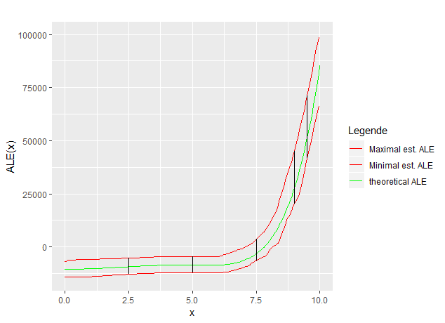
FIGURE 7.5: Maximum range of estimation

The vertical lines indicate the absolute delta of the maximal and minimal ALE estimation at x. Plotting these deltas for the gride sizes 10, 25, and 50 yields Figure 7.6.

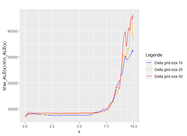
FIGURE 7.6: Delta of maximal and minimal estimated ALE for different grid sizes

It is clearly recognizable that on the one hand for higher x the variance in the ALE estimation increases for all grid sizes. The expected higher variance of the estimations with higher grid sizes is in particular revealed in the region from \(x_1 = 7\) to \(x_1 = 10\), because the estimation is quite sensible to the absolute value of \(x_2\), which also increases with \(x_1\).

As the theoretical ALE in this example was quite smooth, grid size 10 gave reasonable estimations. The following example shows problems that occur once the prediction function is quite shaky especially in regions with only a few observations.

7.1.5 Example 3: Unbalanced datasets and shaky prediction functions

In the 3rd example we assume \(X_1 \sim N(10,3)\) as well as
\(X_2 \vert X_1 = x_1 \sim U(x_1 - 3, x_1 + 3 )\).

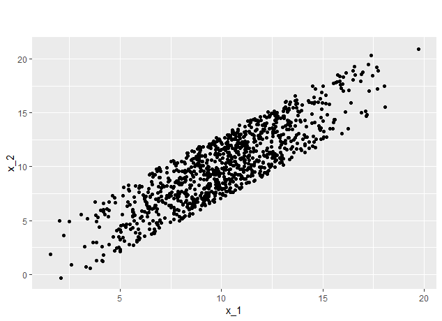
FIGURE 7.7: A mixture of normal and uniform distributed features

For this example the sample size was 1000 (see figure 7.7). As expected the correlation is clearly recognizable. This time only a few data points lay in the outer regions, i.e. between 0 and 2.5 and 17.5 and 20, while there is a high concentration of data around the mean at 10.
Furthermore we look at the prediction function \(\hat{f}_3(x_1,x_2) = sin(10x_1)~x_2\). The calculation of the theoretical uncentered ALE (as before) yields \(~~~~\widetilde{ALE}_{\hat{f},1}(x) = x~sin(x) + \frac{1}{10}cos(10x)\). For centering the expectation of the uncentered ALE, i.e. \(E[\widetilde{ALE}_{\hat{f},1}(X_1)]\), was estimated by Monte-Carlo integration to be almost zero. As well as the prediction function, the theoretical ALE has lots of extreme points. This leads to some troubles, especially for low grid sizes. Figure 7.8 shows the estimated and the theoretical ALE for three different grid sizes.

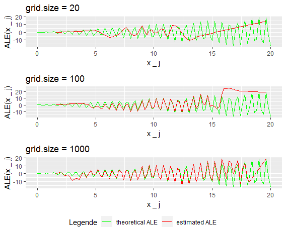
FIGURE 7.8: Theoretical vs. estimated ALE

For grid size 20 the local behavior of the theoretical ALE is absolutely not recognizable. Only one peak left of the mean was estimated reasonable, which is due to the high data intensity in this region. For the rest of the plot, the grid intervals contain two or more peaks. Within each of them, the ALE is estimated linear and therefore the true effect smoothed out.
Increasing the grid size to 100 one nicely sees how the approximation becomes quite reasonable in the inner region, i.e. between 6 and 14, while in the outer region, where the intervals still are too long the ALE continues to be estimated wrong. The more one increases the grid size the wider the inner region of good estimation becomes. Anyway still at grid size 1000 which implies only one data point per interval, the estimations near the boundaries stay bad, as there are simply not sufficient observations to show the fine structure of the prediction function. As this was a constructed example, the latter shouldn't be overrated, as in real data situations it is quite improbable that a learner results in a that granular prediction function within regions with such few data points. While in figure 7.8 apparently both grid sizes (100 and 1000) result in equally good ALE estimations in the inner region, zooming in reveals that this isn't the case.

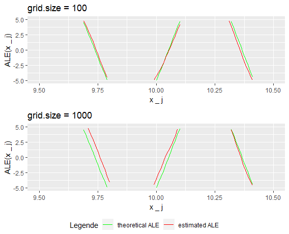
FIGURE 7.9: Zooming in reveals the bias for grid size 1000

Figure 7.9 shows a very small part around the mean. As expected the estimations for grid size 100 are a little closer to the theoretical ALE as again the true effect of the second feature, which still affects the prediction, is better estimated within each interval (10 observations vs 1 observation).

At the end of this section, we have seen a good example of the natural trade-off between small intervals on the one hand and sufficient data to get a good and stable estimation on the other hand. The optimal choice of the number /size of intervals thereby highly depends on the given prediction function and the data. This can be taken as the main message of the section. The next section shall provide the reader with an understanding of how far additional problems can occur in the context of piece-wise constant models.

7.2 Problems with piece-wise constant models

Piece-wise constant models such as for example decision trees and random forests don't have continuous prediction functions, which implies they are not differentiable. Thus the concept of theoretical ALE doesn't make any sense in this context as the partial derivative doesn't exist. Still, it is possible to estimate the ALE as the "jump" will result in a more or less steep linear part, depending on the interval size of the interval containing the step. It is intuitive that the goodness of the estimation highly depends on if one manages to place the intervals quite narrow around the steps. As the following examples will show, problems can occur due to "wrong" interval sizes or unluckily distributed data in the region of the steps.

7.2.1 Example 4: Simple step function

Throughout this section we assume \(X_1\) to be uniformily distributed on the interval \([0,10]\), i.e. \(X_1 \sim U(0,10)\) as well as \(X_2\) given \(X_1\) uniformily on the interval \([max(x_1 - 3, 0),~min( x_1 + 3, 10]]\),
i.e. \(X_2 \vert X_1 = x_1 \sim U(max(x_1 - 3, 0),~min( x_1 + 3, 10) )\). That means all the data is distributed within the 10 times 10 square. In the first example, we take a look at a simple prediction function to get a good understanding of the basic problem with piece-wise constant models. We assume a prediction function that independently of \(x_2\) predicts 0, except if \(x_1\) falls into a certain small interval around 5. In this case, it predicts 10. Concretely \(f(x_1, x_2) = 1_{[4.9,~5.1]}(x_1) * 10\).

Figure 7.10 shows a sampled data set of 100 data points and a sketch of the prediction function.

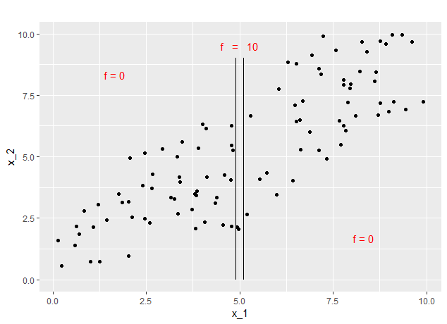
FIGURE 7.10: Prediction Function 1

As mentioned above a good estimation of the ALE would result in quite steep linear parts, one around 4.9 and a second inverse one around 5.1. The problem now is that the ALE estimation won't catch those jumps as long as both jumps lay within the same interval. The reason is that all the points within this interval would be moved to the interval boundaries which lay outside the area, where the prediction function predicts 10. This leads to an estimation of the local effect as zero. Figure 7.11 shows the estimates for different grid sizes 20, 30, 50 and 100.

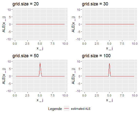
FIGURE 7.11: The behavior of ALE estimation with increasing grid size

As expected the ALE estimations with grid size 20 and 30 are not sensitive to the effect. Increasing the grid size ensures that some interval boundaries fall into the interval \([4.9, ~5.1]\) which exposes the step of the prediction function. Having a second look at the data situation in this example, one notes that only 2 data points fall to the interval \([4.9, ~5.1]\). Grid size 50 implies for 100 datapoints 2 data points per interval. That means that we even got lucky in this example that the 2 data points didn't fall into the same grid interval. Otherwise, the effect would have remained hidden even at grid size 50. The following example shows how unluckily distributed data points can lead to bad ALE estimations.

7.2.2 Example 5: Two-dimensional step functions and unluckily distributed data

We assume the same data distribution as in the former example. Furthermore well take a look on two prediciton functions, one independent of \(x_2\) defined as \(f(x_1, x_2) = 1 + 1_{[0,~\frac{10}{3}]}(x_1)+ 1_{[\frac{10}{3},~\frac{20}{3}]}(x_1)\). The second also depends on \(x_2\) and is defined as \(f(x_1, x_2) = 3~(1_{[\frac{10}{3},~\frac{20}{3}]}(x_1)~*~1_{[\frac{10}{3},~\frac{20}{3}]}(x_2)) + 2~(1_{[0,~\frac{10}{3}]}(x_1)~*~(1_{[0,~\frac{10}{3}]}(x_2)+1_{[\frac{20}{3}, ~10]}(x_2)) + ~(1_{[\frac{20}{3},~10]}(x_1)~*~(1_{[0,~\frac{10}{3}]}(x_2)+1_{[\frac{20}{3}, ~10]}(x_2))\) . Both on the first sight a little unhandy become quite easy to understand looking at the sketches below (see figures 7.12 and 7.13).

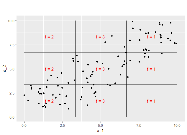
FIGURE 7.12: Prediction function 2

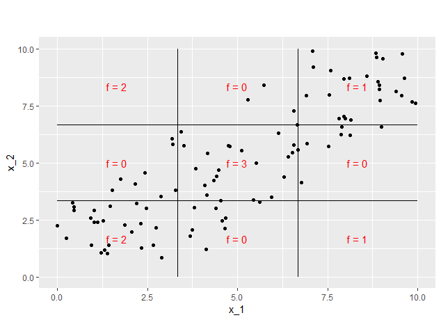
FIGURE 7.13: Prediction function 3

In the following, the ALE was estimated for increasing grid sizes. In figure 7.14 starting with grid size 5 on the left side we see the behavior of the first prediction function on the right side for the second one.

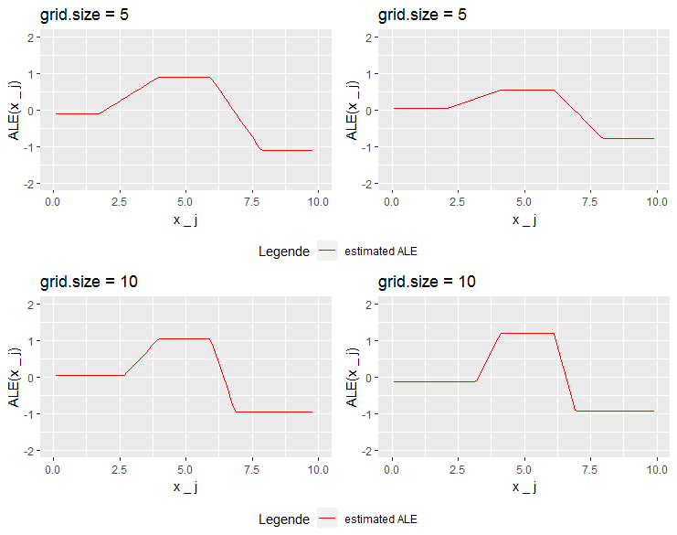
FIGURE 7.14: Behaviour of ALE estimations for prediction function 2 (leftside) and 3 (rightside)

For grid size 5 both estimations recognize the step but estimate it relatively flat, which is not very surprising as the interval length should be around 2. For the first prediction function, we see a total increase within the second grid interval of 1 and a total decrease in the fourth one of 2. This reflects the behavior of the prediction function, so the only problem is the low grid size. For the second prediction functions, the total changes are estimated to be much lower. This is due to the areas of 0 prediction which clearly influence the mean change in prediction, as some data points change from 0 to 3, but others from 2 to 0 within the second grid interval, as well as from 3 to 0 and from 0 to 1 within the fourth grid interval. So the absolute effect of \(x_1\) is relativized by the influence of \(x_2\), which is intended by the concept of ALE. At grid size 10 the estimations for both prediction functions look quite similar. The steps become steeper as the grid intervals shrink to half their length. The estimated change in prediction for the second prediction function now is even bigger than for the first one. Due to the correlation, now more (relatively more) datapoints are shifted from prediction 0 to 3 and 3 to 0 respectively, which leads to the slightly higher estimation of the effect.

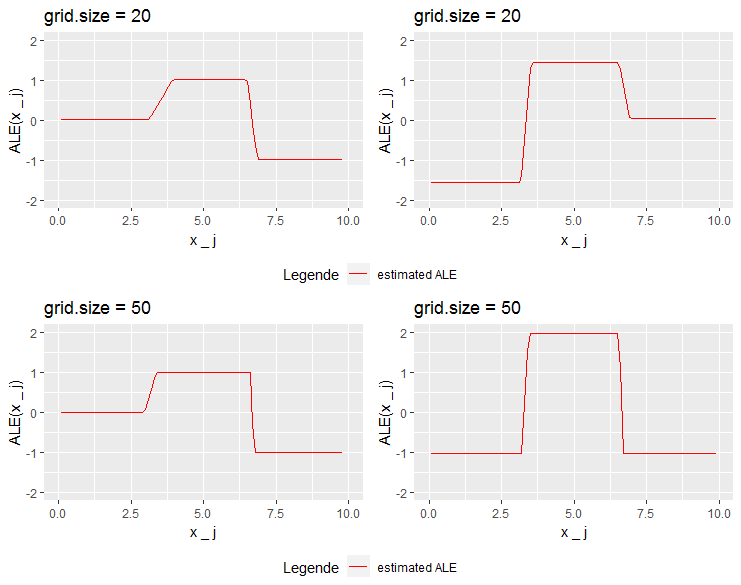
FIGURE 7.15: Behaviour of ALE estimations for prediction function 2 (leftside) and 3 (rightside)

Increasing the grid size first to 20 and then to 50 reveals the whole danger of this situation. While prediction function 2 seems to be estimated quite stable (the absolute changes stay to be 1 and -2, while the steps become steeper and steeper), the estimation for prediction function 3 changes its behavior. At grid size 20 the left step grows to be 3, at grid size 50 the second step to be -3. Centering leads to quite radical upwards and downwards shifts of the whole plot. To understand this we'll have a look at the data points that are used to estimate the steps.

FIGURE 7.16: Points that are used to estimate the step at grid size 20

For grid size 20, 5 data points are used to estimate the total change in prediction. As figure 7.16 shows, coincidentally 5 data points with \(x_2\)-values between \(\frac{10}{3}\) and \(\frac{20}{3}\) fall into the step interval. This is why the mean difference of the prediction is estimated to be 3.

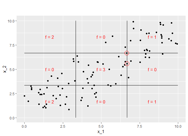
FIGURE 7.17: Points that are used to estimate the step at grid size 50

Analogously for grid size 50, only two data points are used. As again both fall into the same \(x_2\) - range, the estimation of the mean change of prediction in this grid interval is -3 now. Looking at figure 7.17 it becomes clear that only a little higher \(x_2\) value of the upper data point would have lead to an estimation of -1 instead. This shows how sensitive the ALE estimation in the context of piece-wise constant models is. While there could be arguments for the height of the steps in the first 3 estimations, the last estimation clearly displays a false image. Here the interpretation would be that there is no main effect of feature 1 changing from less than \(\frac{10}{3}\) to higher than \(\frac{20}{3}\), which is obviously wrong.

7.2.3 Outlook

We have seen that ALE estimations in the context of piece-wise constant models are even more critical due to sharp changes in the prediction at the steps. On the one hand, one needs the intervals to be within the steps to recognize them and at the same time quite narrow around them to catch the steepness of the step. Notice that in real-world examples one cannot know if there is a step or if the flat linear approximation is true. On the other hand, the data distribution around the steps has a strong influence on the ALE which leads to highly unstable estimations. In this context different methods of interval selection, maybe even adaptive, data-driven methods should be investigated.

7.3 Categorical Features

So far we were only interested in ALE-estimations for a numerical feature of interest. In real data situations, categorical features often play an important role. That's why it would be nice to expand the concept of ALE so that it can also be applied to categorical features. In the original paper by (Apley 2016) this concept was not described but still, the first method implemented. (Molnar 2019) adapted the method for the iml-package. The following section briefly describes the implemented method as well as the interpretation of ALE-plots for categorical features. It also shows some specific problems.

7.3.1 Ordering the features

One of the biggest and crucial differences of categorical and numerical features in the context of ALE is that categorical features usually don't have a natural order. As the concept of ALE is based on accumulating the local effects in a certain direction, an order of the feature is indispensable. Sometimes the categorical feature is an ordinal feature that comes with a natural order. In this case, the natural order should be used. If there is no natural order, the first essential step to calculate the ALE is to order the feature. Therefore different methods are conceivable. The iml-package implementation tries to order the feature with respect to the similarity of the other features. As we'll see in the next subsection for the estimation of the ALE the data points of a category will be shifted to the neighbor categories (neighbor categories only exist if the feature is ordered). To stay with the original idea of ALE and try to avoid extrapolation, ordering the feature with respect to the similarity of the other features seems reasonable. Within the iml-package, in a first step, the distance of each pair of categories (of the feature of interest) is calculated with respect to every other feature. This results in \(\frac{c~(c-1)~(f-1)}{2}\) distances, where f is the total number of features while c is the number of categories of the feature of interest. To calculate these distances for numerical features the Kolmogorov-Smirnov distance is used. It is defined as the maximal absolute difference of two distribution functions, which are estimated from the data within the two compared categories. For categorical features, one simply sums up the absolute differences of the relative frequencies of the categories. Finally, the distance between the two categories is calculated as the sum of their distances with respect to all features. Once the distance between all categories is calculated, multidimensional scaling is used to reduce the distance matrix to a one-dimensional distance measure (Molnar 2019).

7.3.2 Estimation of the ALE

Once the features are ordered (no matter if as proposed by (Apley 2016) and (Molnar 2019) or in a different order) it's still not clear how to estimate the ALE. The partitioning of the axis into intervals doesn't make sense anymore as the categories themselves kind of partition the range of the feature in a natural manner. But there are no "values" in-between them and at the same time, the data points fall exactly on them. A continuous ALE wouldn't make sense at all, as there are no possibilities of changing the feature value if not from one category to another category. That's why the idea is to estimate exactly these expected changes in prediction if one category is changed to its neighbor category. Therefore for each pair of neighbor categories, the expected change is estimated by shifting the data from the lower to the upper category and vice verse and calculating the mean difference of the prediction. This mean difference is taken to be the expected effect between these two categories. How these changes are accumulated and how the ALE-plot looks, becomes clearer once looking at an example.

7.3.3 Example of ALE with categorical feature

For the following example the Munich rent dataset, which consists of a sample of 2053 apartments from the data collected for the preparation of the Munich rent index 2003, was used. For our purposes we restricted the data to the variables rentm (Net rent per square meter in EUR (numeric)), size (Floor area in square meters (numeric)), rooms (Number of rooms (numeric)), year (Year of construction (numeric)) and area (Urban district where the apartment is located (Factor with 25 levels)). In the first step, a model (Support Vector Machine for Regression) was fitted to predict the variable rentm. Now the ALE for the feature area, which is a categorical variable, was estimated with the iml-package. Figure 7.18 shows the result.

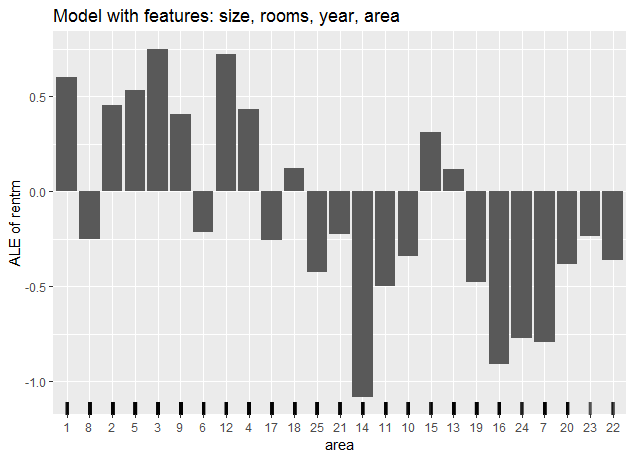
FIGURE 7.18: ALE for the variable area (categorical)

As described previously in a first step the categories (each number stands for one district) were ordered on basis of their similarity w.r.t. the other features. Notice that the first bar at category one only reflects the centering. The uncentered ALE wouldn't show an effect on this category as it is kind of the starting point. Now the mean difference of prediction between category 1 and 8 was calculated. Therefore datapoints from category 1 were shifted to category 8, letting the rest of the features untouched and vice versa. The total effect was estimated as the mean difference in prediction for these data points. It is shown as the delta of the category 1 bar and the category 8 bar. Without centering it would be seen at the category 8 bar. Now the same difference is estimated for the change from category 8 to category 2 and is shown as the delta of their bars. This procedure continues until finally the change from category 23 to category 22 results in the last delta between their bars.

7.3.4 Interpretation

The interpretation of the ALE-plot for categorical features is unfortunately quite difficult. The deltas between two adjacent bars surely can be interpreted as the change between the corresponding categories. Once looking at deltas of two categories with one or more other categories in between, this changes. The delta is not any longer the change of prediction between the two categories but the estimated change of prediction for shifting through all the categories in between in exactly the given order. The reason is that the estimated delta is not path independent. For example, the delta between categories 1 and 2 in the example above was calculated using data points of category 1, 8, and 2. If they were direct neighbors, the data points of category 8 wouldn't be involved in the estimation at all. This problem clearly grows the further two categories are ordered. Having this in mind the absolute values of the bars shouldn't be interpreted at all. Furthermore, this is another argument for ordering the categories in a reasonable manner, while it stays arguable what "reasonable" in this context means.

7.3.5 Changes of the ALE due to different orders

The last two graphics show how much the ALE for categorical features depends on the underlying order of the features. For the first one, the same learner was fitted on a restricted feature space containing only the variables year and area.

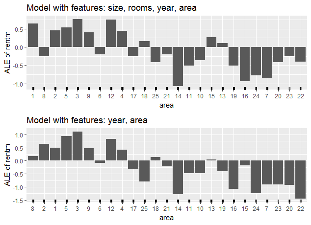
FIGURE 7.19: ALE-plot of the full model vs ALE-plot of the restricted model

As the comparison of the ALE-plots of figure 7.19 shows, the similarity-based order changes as it is only calculated on basis of the variable year (instead of size, room, year). As the underlying model is now a different one, changes in the ALE are not surprising. Still, the comparison is quite difficult due to the new order.

The second ALE-plot of figure 7.20 is again based on the full model. This time the area was taken as an ordered factor, such that the similarity-based order wasn't calculated. The resulting ALE takes the district enumeration as order and proceeds accordingly.

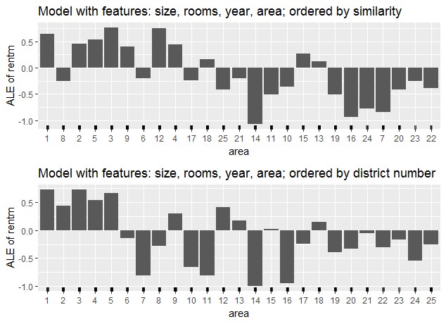
FIGURE 7.20: Two ALE-plots for different orders of the category area

Although the underlying model is the same, the ALE changes completely. Not only the order of the features changed but also the delta between some not adjacent categories. For example, we see a decrease from category 1 to 12 instead of an increase, as in the ALE-plot with similarity-based order. This underlines how careful one should be when interpreting ALE-plots for categorical features.

7.3.6 Conclusion

We have seen how sensitive the ALE (for categorical features) is for different orders of the category. Due to the lack of theoretical foundations concerning the implemented order method, further investigations are highly recommended. The interpretation of the ALE should be done quite carefully.

References

Apley, Daniel W. 2016. Visualizing the Effects of Predictor Variables in Black Box Supervised Learning Models. https://arxiv.org/ftp/arxiv/papers/1612/1612.08468.pdf.

Molnar, Christoph. 2019. Interpretable Machine Learning: A Guide for Making Black Box Models Explainable.