Chapter 3 PDP and Correlated Features

Author: Veronika Kronseder

Supervisor: Giuseppe Casalicchio

3.1 Problem Description

As outlined in chapter 2, PDPs and ICE plots are meaningful graphical tools to visualize the impact of individual feature variables. This is particularly true for black box algorithms, where the mechanism of each feature and its influence on the generated predictions may be difficult to retrace (Goldstein et al. 2013).

The reliability of the produced curves, however, strongly builds on the independence assumption of the features. Furthermore, results can be misleading in areas with no or little observations, where the curve is drawn as a result of extrapolation. In this chapter, we want to illustrate and discuss the issue of dependencies between different types of variables, missing values and the associated implications on PDPs.

3.1.1 What is the issue with dependent features?

When looking at PDPs, one should bear in mind that by definition the partial dependence function does not reflect the isolated effect of $x_S$ while the features in $x_C$ are ignored. This approach would correspond to the conditional expectation $\tilde{f}_S(x_S) = \mathbb{E}_{x_C}[f(x_S, x_C)|x_S]$, which is only congruent to the partial dependence function $f_{x_S}(x_S) = \mathbb{E}_{x_C}[f(x_S, x_C)]$ in case of $x_S$ and $x_C$ being independent (Hastie, Tibshirani, and Friedman 2013).

Although unlikely in many practical applications, the independence of feature variables is one of the major assumptions to produce meaningful PDPs. Its violation would mean that, by calculating averages of the features in $x_C$, the estimated partial dependence function $\hat{f}_{x_S}(x_S)$ takes unrealistic data points into consideration (Molnar 2019).

Figure 3.1 illustrates the problem by contrasting simulated data with independent features $x_1$ and $x_2$ on the left with an example where the two features have a strong linear dependency, and thus are highly correlated, on the right.

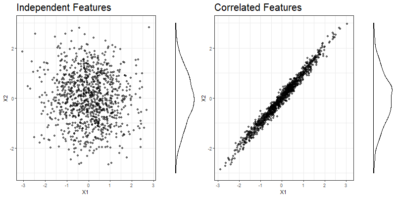
Simulated data for independent (left) and strongly correlated (right) features $x_1$ and $x_2$. The marginal distribution of $x_2$ is displayed on the right side of each plot.

FIGURE 3.1: Simulated data for independent (left) and strongly correlated (right) features $x_1$ and $x_2$. The marginal distribution of $x_2$ is displayed on the right side of each plot.

When computing the PDP for feature $x_1$, we take $x_2$ into account by calculating the mean predictions at observed $x_2$ values in the training data, while the values of $x_1$ are given. This makes sense in the independent case, where observations are randomly scattered. However, when looking at the correlated features in the right part of figure 3.1, the average is not a realistic value in combination with certain values of $x_1$, e.g. in the very left and the very right part of the feature distribution.

3.1.2 What is the issue with extrapolation?

Generally speaking, extrapolation means leaving the distribution of observed data. On the one hand, this can affect the predictions, namely in the event of the prediction function doing 'weird stuff' in unobserved areas. In chapter 3.4 we will see an example where this instant leads to a failure of the PDP (Molnar 2019).

On the other hand, PDPs are also directly exposed to extrapolation problems due to the fact that the estimated partial dependence function $\hat{f}_{x_S}$ is evaluated at each observed $x^{(i)}_{S}$, giving a set of N ordered pairs: $\{(x^{(i)}_{S}, \hat{f}_{x^{(i)}_{S}})\}_{i=1}^N$. The resulting coordinates are plotted against each other and joined by lines. Not only outside the margins of observed values, but also in areas with a larger distance between neighboured $x_S$ values, the indicated relationship with the target variable might be inappropriate and volatile in case of outliers (Goldstein et al. 2013).

In figure 3.2, a part of the previously simulated observations has been deleted from both the independent and the correlated example to visualize a data situation which might have an impact on the PDP in terms of extrapolation. An example is given in chapter 3.4.1. The shift in observed areas can also be noticed from the marginal distribution of $x_2$.

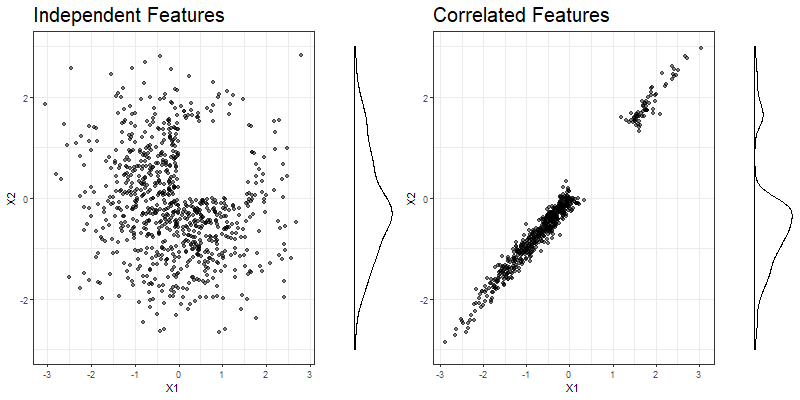
Manipulated simulated data for independent (left) and strongly correlated (right) features $x_1$ and $x_2$. Observations where both the value of $x_1$ and $x_2$ lies between 0 and 1.5 have been deleted to artificially produce an extrapolation problem. The marginal distribution of $x_2$, which is displayed on the right side of each plot, is obviously more affected in the correlated case.

FIGURE 3.2: Manipulated simulated data for independent (left) and strongly correlated (right) features $x_1$ and $x_2$. Observations where both the value of $x_1$ and $x_2$ lies between 0 and 1.5 have been deleted to artificially produce an extrapolation problem. The marginal distribution of $x_2$, which is displayed on the right side of each plot, is obviously more affected in the correlated case.

The extrapolation problem in PDPs is strongly linked to the aforementioned independence assumption. Independent features are a prerequisite for the computation of meaningful extrapolation results, therefore one could say that both problems go hand in hand. In the following chapters, the failure of PDPs in case of a violation of the independence assumption shall be discussed by means of real data examples (chapter 3.2) and based on simulated cases (chapter 3.3).

3.2 Dependent Features: Bike Sharing Dataset

In order to investigate the impact of dependent features, we are now looking at the Bike-Sharing dataset from the rental company 'Capital-Bikeshare', which is available for download via the UCI Machine Learning Repository. Besides the daily count of rental bikes between the year 2011 and 2012 in Washington D.C., the dataset contains the corresponding weather and seasonal information (Fanaee-T and Gama 2013).

For our purposes, the dataset was restricted to the following variables:

$y$: cnt (count of total rental bikes including both casual and registered)
$x_1$: season: Season (1:springer, 2:summer, 3:fall, 4:winter)
$x_2$: yr: Year (0: 2011, 1:2012)
$x_3$: mnth: Month (1 to 12)
$x_4$: holiday: weather day is holiday or not
$x_5$: workingday: If day is neither weekend nor holiday is 1, otherwise is 0.
$x_6$: weathersit:
- 1: Clear, Few clouds, Partly cloudy, Partly cloudy
- 2: Mist + Cloudy, Mist + Broken clouds, Mist + Few clouds, Mist
- 3: Light Snow, Light Rain + Thunderstorm + Scattered clouds, Light Rain + Scattered clouds
- 4: Heavy Rain + Ice Pallets + Thunderstorm + Mist, Snow + Fog
$x_7$: temp: Normalized temperature in Celsius.
$x_8$: atemp: Normalized feeling temperature in Celsius.
$x_9$: hum: Normalized humidity.
$x_{10}$: windspeed: Normalized wind speed.

For all machine learning models based on the Bike-Sharing dataset, 'cnt' is used as a target variable, while the remaining information serves as feature variables. Six out of these ten features are categorical ($x_1$ to $x_6$), the rest is measured on a numerical scale ($x_7$ to $x_{10}$). Since the appearance of a PDP depends on the class of the feature(s) of interest, we are looking at three different scenarios of dependency:

Dependency between numerical features
Dependency between categorical features
Dependency between numerical and categorical features

At the same time, for each of those scenarios, three different learning algorithms shall be compared:

Linear Model (LM)
Random Forest (RF)
Support Vector Machines (SVM)

3.2.1 Dependency between Numerical Features

The linear dependency between two numerical features can be measured by the Pearson correlation coefficient (Fahrmeir et al. 2016). Figure 3.3 shows the correlation matrix of all numerical features used in our analysis. It is striking, but certainly not surprising, that 'temp' and 'atemp' are strongly correlated, not to say almost perfectly collinear.

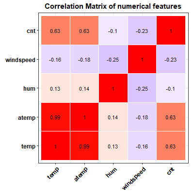
FIGURE 3.3: Matrix of Pearson correlation coefficients between all numerical variables extracted from the bike-sharing dataset.

Due to their strong correlation, 'temp' ($x_7$) and 'atemp' ($x_8$) perfectly qualify for our analysis of the impact of dependent features on PDPs. In order to compare the partial dependence curve with and without the influence of dependent features, we compute PDPs based on the following models:

\[\begin{equation} y \sim x_1 + x_2 + x_4 + x_5 + x_6 + \mathbf{x_7} + x_9 + x_{10} \tag{3.1} \end{equation}\] \[\begin{equation} y \sim x_1 + x_2 + x_4 + x_5 + x_6 + \mathbf{x_8} + x_9 + x_{10} \tag{3.2} \end{equation}\] \[\begin{equation} y \sim x_1 + x_2 + x_4 + x_5 + x_6 \mathbf{+ x_7 + x_8} + x_9 + x_{10} \tag{3.3} \end{equation}\]

Please note that the representation of the different models with the feature variables connected via '+' shall, in this context, not be read as a (linear) regression model where all coefficients are equal to 1, but rather as a combination of applicable feature variables to explain $y$. The (non-)linear effect of each variable is modelled individually, depending on the observed values and the learner.

While model (3.1) and (3.2) only take one of the two substituting variables into account, (3.3) considers both 'temp' and 'atemp' in one and the same model. Figures 3.4, 3.5 and 3.6 compare the associated PDPs for the different learning algorithms. Note that 'season' ($x_1$) and 'mnth' ($x_3$) are not taken into account in combination with $x_7$ and/or $x_8$, since there are meaningful associations between those variables, too, as we will show in chapter 3.2.3. At this stage we want to illustrate the isolated effect of the dependence between the two numerical variables.

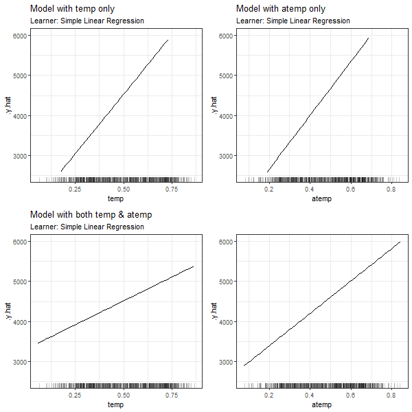
PDPs based on Linear Regression learner for 'temp' in model 3.1 (top left), 'atemp' in model 3.2 (top right), 'temp' in model in model 3.3 (bottom left) and 'atemp' in model 3.3 (bottom right).

FIGURE 3.4: PDPs based on Linear Regression learner for 'temp' in model 3.1 (top left), 'atemp' in model 3.2 (top right), 'temp' in model in model 3.3 (bottom left) and 'atemp' in model 3.3 (bottom right).

PDPs based on Support Vector Machines learner for 'temp' in model 3.1 (top left), 'atemp' in model 3.2 (top right), 'temp' in model in model 3.3 (bottom left) and 'atemp' in model 3.3 (bottom right).

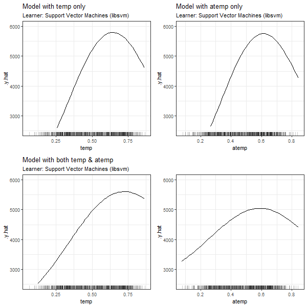
FIGURE 3.5: PDPs based on Support Vector Machines learner for 'temp' in model 3.1 (top left), 'atemp' in model 3.2 (top right), 'temp' in model in model 3.3 (bottom left) and 'atemp' in model 3.3 (bottom right).

PDPs based on Random Forest learner for 'temp' in model 3.1 (top left), 'atemp' in model 3.2 (top right), 'temp' in model in model 3.3 (bottom left) and 'atemp' in model 3.3 (bottom right).

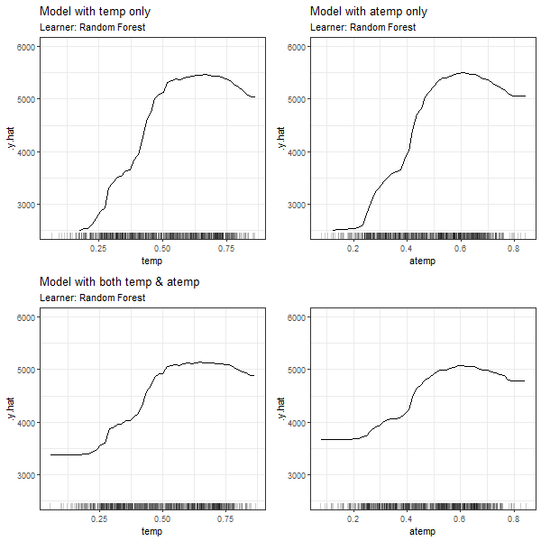
FIGURE 3.6: PDPs based on Random Forest learner for 'temp' in model 3.1 (top left), 'atemp' in model 3.2 (top right), 'temp' in model in model 3.3 (bottom left) and 'atemp' in model 3.3 (bottom right).

In all cases, we can see that the features' effect on the prediction is basically the same for $x_7$ and $x_8$, if only one of the dependent variables is used for modelling (see PDPs in top left and top right corners). If both 'temp' and 'atemp' are relevant for the prediction of $y$, each feature's impact is smoothened and neither the PDP for $x_7$ nor the one for $x_8$ seems to properly reflect the true effect of the temperature on the count of bike rentals.

3.2.2 Dependency between Categorical Features

In order to measure the association between two categorical features, we calculate the corrected contingency coefficient, which is based on the $\chi^2$-statistic. Other than the Pearson correlation coefficient, the corrected contingency coefficient is a measure of association $\in [0,1]$ which can only indicate the strength but not the direction of the variables' relationship (Fahrmeir et al. 2016). For the categorical features in the Bike-Sharing dataset, we observe the values stated in figure 3.7.

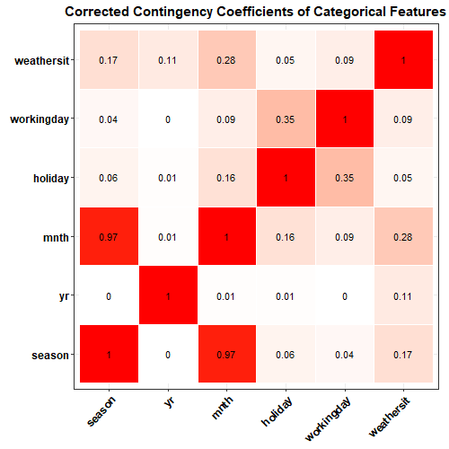
FIGURE 3.7: Matrix of corrected contingency coefficients between all categorical variables extracted from the bike-sharing dataset.

The only combination of categorical features with an exceptionally high corrected contingency coefficient, is 'season' ($x_1$) and 'mnth' ($x_3$). Also from a content-related point of view, this finding is no surprise, since both variables measure the time of the year. For the computation of the respective PDPs, we use the following models:

\[\begin{equation} y \sim \mathbf{x_1} + x_2 + x_4 + x_5 + x_6 + x_9 + x_{10} \tag{3.4} \end{equation}\] \[\begin{equation} y \sim x_2 +\mathbf{x_3} + x_4 + x_5 + x_6 + x_9 + x_{10} \tag{3.5} \end{equation}\] \[\begin{equation} y \sim \mathbf{x_1} + x_2 + \mathbf{x_3} + x_4 + x_5 + x_6 + x_9 + x_{10} \tag{3.6} \end{equation}\]

The approach is equivalent to the numeric case, with model (3.4) containing only 'season' and (3.5) only 'mnth', while both dependent features are part of model (3.6). The impact on the PDPs for categorical features are shown in figures 3.8, 3.9 and 3.10.

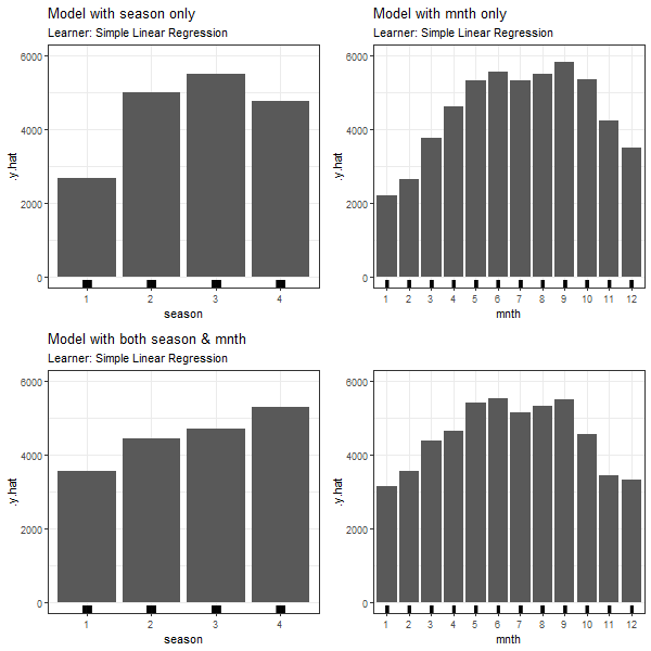
PDPs based on Linear Regression learner for 'season' in model 3.4 (top left), 'mnth' in model 3.5 (top right), 'season' in model in model 3.6 (bottom left) and 'mnth' in model 3.6 (bottom right).

FIGURE 3.8: PDPs based on Linear Regression learner for 'season' in model 3.4 (top left), 'mnth' in model 3.5 (top right), 'season' in model in model 3.6 (bottom left) and 'mnth' in model 3.6 (bottom right).

PDPs based on Support Vector Machines learner for 'season' in model 3.4 (top left), 'mnth' in model 3.5 (top right), 'season' in model in model 3.6 (bottom left) and 'mnth' in model 3.6 (bottom right).

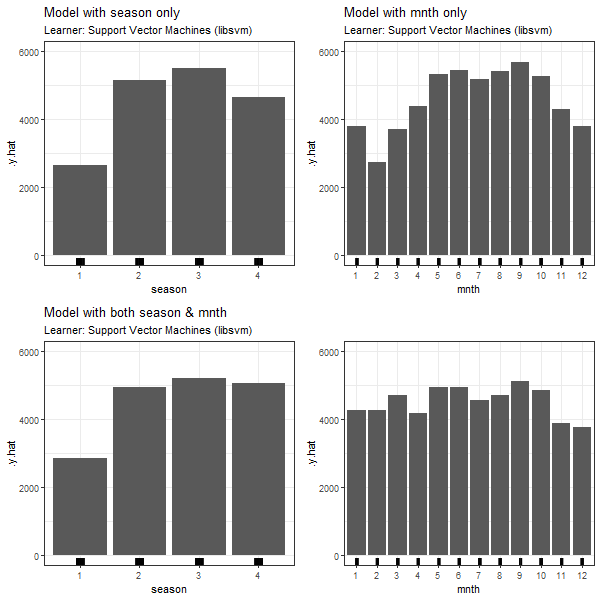
FIGURE 3.9: PDPs based on Support Vector Machines learner for 'season' in model 3.4 (top left), 'mnth' in model 3.5 (top right), 'season' in model in model 3.6 (bottom left) and 'mnth' in model 3.6 (bottom right).

PDPs based on Random Forest learner for 'season' in model 3.4 (top left), 'mnth' in model 3.5 (top right), 'season' in model in model 3.6 (bottom left) and 'mnth' in model 3.6 (bottom right).

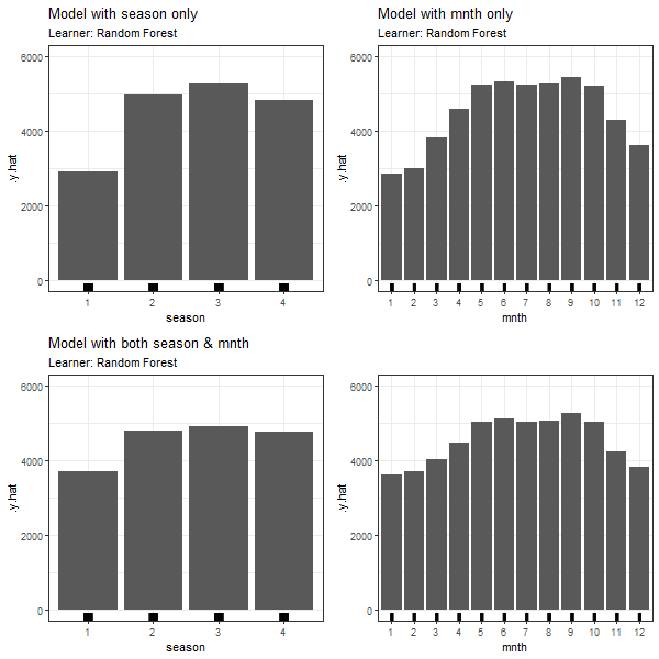
FIGURE 3.10: PDPs based on Random Forest learner for 'season' in model 3.4 (top left), 'mnth' in model 3.5 (top right), 'season' in model in model 3.6 (bottom left) and 'mnth' in model 3.6 (bottom right).

Again, in all PDPs based on the different learning algorithms, the results between models with and without dependent features are diverging. The predicted number of bike rentals between the seasons/months shows a stronger variation when modelled without feature dependencies.

3.2.3 Dependency between Numerical and Categorical Features

Our third dependency scenario seeks to provide an example for a strong correlation between a numerical and a categorical feature. For this constellation, neither the Pearson correlation nor the contingency coefficient are applicable as such, since both methods are limited to their respective classes of variables.

We can, however, fit a linear model to explain the numeric variable through the categorical feature. By doing so, we produce another numerical variable, the fitted values. In a next step, we can calculate the Pearson correlation coefficient between the observed and the fitted values of the numerical feature. The resulting measure of association lies within the interval $[0,1]$ and is equivalent to the square root of the linear model's variance explained ($R^2$) (Fahrmeir et al. 2013). For this reason, we refer to the measure as 'variance-explained measure'.

When applying this procedure to the categorical feature 'season' ($x_1$) and the numerical feature 'temp' ($x_7$), we find that with a variance-explained value of 0.83, there seems to be a reasonable association between the two features. The PDPs are derived through the following models:

\[\begin{equation} y \sim \mathbf{x_1} + x_2 + x_4 + x_5 + x_6 + x_9 + x_{10} \tag{3.7} \end{equation}\] \[\begin{equation} y \sim x_1 + x_2 + x_4 + x_5 + x_6 + \mathbf{x_7}+ x_9 + x_{10} \tag{3.8} \end{equation}\] \[\begin{equation} y \sim \mathbf{x_1} + x_2 + x_4 + x_5 + x_6 +\mathbf{x_7}+ x_9 + x_{10} \tag{3.9} \end{equation}\]

Figure 3.11, 3.12 and 3.13 present the partial dependence plots for the three underlying machine learning algorithms (LM, SVM and RF) defined for the purpose of our analysis.

PDPs based on Linear Regression learner for 'season' in model 3.4 (top left), 'temp' in model 3.5 (top right), 'season' in model in model 3.6 (bottom left) and 'temp' in model 3.6 (bottom right).

FIGURE 3.11: PDPs based on Linear Regression learner for 'season' in model 3.4 (top left), 'temp' in model 3.5 (top right), 'season' in model in model 3.6 (bottom left) and 'temp' in model 3.6 (bottom right).

PDPs based on Support Vector Machines learner for 'season' in model 3.4 (top left), 'temp' in model 3.5 (top right), 'season' in model in model 3.6 (bottom left) and 'temp' in model 3.6 (bottom right).

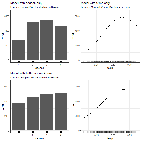
FIGURE 3.12: PDPs based on Support Vector Machines learner for 'season' in model 3.4 (top left), 'temp' in model 3.5 (top right), 'season' in model in model 3.6 (bottom left) and 'temp' in model 3.6 (bottom right).

PDPs based on Random Forest learner for 'season' in model 3.4 (top left), 'temp' in model 3.5 (top right), 'season' in model in model 3.6 (bottom left) and 'temp' in model 3.6 (bottom right).

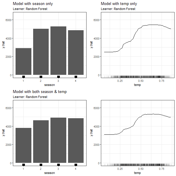
FIGURE 3.13: PDPs based on Random Forest learner for 'season' in model 3.4 (top left), 'temp' in model 3.5 (top right), 'season' in model in model 3.6 (bottom left) and 'temp' in model 3.6 (bottom right).

Compared to the first two scenarios, we observe a more moderate difference between the PDPs when comparing model (3.7) and (3.8) containing just one of the dependent features to the full model (3.9). The weaker association between the two variables, in contrast to scenario 1 and 2, could be an explanation for this observation. It is, however, evident that the dependency structure between two feature variables, irrespective of their class, does impact the partial dependence plot.

3.3 Dependent Features: Simulated Data

A major disadvantage of the analysis of PDPs on the basis of real data examples is, that we cannot exclude other factors to play a role. As an example, underlying interactions could have an impact on the PDP and hide the true effect of a feature on the predicted target variable (Molnar 2019). In order to illustrate the isolated impact of dependent variables in the feature space, we have simulated data in different settings, which we will discuss in this chapter.

3.3.1 Simulation Settings: Numerical Features

For a start, the different settings of simulations used for our investigation shall be introduced. Just like in chapter 2, we are separately looking at different classes of variables and different machine learning algorithms (LM, RF and SVM). PDPs for independent, correlated and dependent numerical features are computed for each of the following data generating processes (DGP), which describe the true impact of the features on $y$:

Setting 1: Linear Dependence:
\[\begin{equation} y = x_1 + x_2 + x_3 + \varepsilon \tag{3.10} \end{equation}\]
Setting 2: Nonlinear Dependence in $x_1$:
\[\begin{equation} y = \sin{( \, 3*x_1 ) \,} + x_2 + x_3 + \varepsilon \tag{3.11} \end{equation}\]
Setting 3: Missing informative feature $x_3$
\[\begin{equation} y = x_1 + x_2 + x_3 + \varepsilon \tag{3.12} \end{equation}\] with $x_3$ relevant for the DGP but unconsidered in the machine learning model.

In the independent case, the feature variables $x_1$, $x_2$ and $x_3$ have been drawn from a gaussian distribution with $\mu = 0$, $\sigma^2 = 1$ and a correlation coefficient of $\rho_{ij} = 0$ $\forall$ $i \ne j$, $i,j \in \{1,2,3\}$.
The correlated case is based on the same parameters for $\mu$ and $\sigma^2$, but a correlation coefficient of $\rho_{12} = \rho_{21} = 0.90$, i.e. a relatively strong linear association between $x_1$ and $x_2$, and $\rho_{ij} = 0$ otherwise.
The dependent case describes the event of perfect multicollinearity, where $x_2$ is a duplicate of $x_1$, based on the data generated in the independent case.
The target variable $y$ results from the respective DGP with an error term $\varepsilon \sim N(0, \sigma^2_\varepsilon)$ and $\sigma^2_\varepsilon$ depending on the feature values.

One source of variation in the PDPs is the simulation of the data itself. For this reason, the process has been repeated 20 times for each analysis and the resulting PDP curves are shown as gray lines in the plots below. The thicker, black line represents the average partial dependence curve over these 20 simulations and the error bars indicate their variation. Additionally, a red line represents the true effect of the feature for which the PDP is computed. In all cases, the simulations are based on a number of 500 observations and grid size 50.

Since in the dependent case, $x_2$ is simply a duplicate of $x_1$, the DGP could also be written as $y = 2*x_1 + x_3 + \varepsilon$ in setting (3.10) and (3.12) and $y = \sin{( \, 3*x_1 ) \,} + x_1 + x_3 + \varepsilon$ in setting (3.11). For the purpose of this analysis, we are looking at each of the three features' PDP separately. However, in order to illustrate the aforementioned, the common effect of $x_1$ and $x_2$ on the prediction is added to the plots as dashed blue line.

3.3.2 Simulation of Setting 1: Linear Dependence

3.3.2.1 PDPs based on Linear Model

The results of our simulations in setting 1 based on the Linear Model are shown in figure 3.14:

PDPs for features $x_1$, $x_2$ and $x_3$ (left to right) in Setting 1, based on multiple simulations with Linear Model as learning algorithm. Top row shows independent case, second row the correlated case and bottom row the dependent case. The red line represents the true effect of the respective feature on $y$, the blue dashed line is the true commmon effect of $x_1$ and $x_2$.

FIGURE 3.14: PDPs for features $x_1$, $x_2$ and $x_3$ (left to right) in Setting 1, based on multiple simulations with Linear Model as learning algorithm. Top row shows independent case, second row the correlated case and bottom row the dependent case. The red line represents the true effect of the respective feature on $y$, the blue dashed line is the true commmon effect of $x_1$ and $x_2$.

Across all simulations, there is hardly any variation between the PDPs based on the Linear Model. In the independent case, the PDPs for each feature adequately reflect the linear dependency structure. The effect is equivalent in each PDP, since all features have the same impact and are independent from each other. From the PDPs in the second row of figure 3.14 we see that even with a relatively strong correlation of features $x_1$ and $x_2$, the PDPs adequately reflect the linear dependency structure when predictions are computed from the Linear Model. In the event of perfect multicollinearity, the PDP for one of the dependent features ($x_2$) fails, while the corresponding PDP for the other feature ($x_1$) reflects the common effect of both. The PDP for feature $x_3$ adequately reveals its linear effect on $y$.

3.3.2.2 PDPs based on Random Forest

The results of our simulations in setting 1 based on Random Forest are shown in figure 3.15:

PDPs for features $x_1$, $x_2$ and $x_3$ (left to right) in Setting 1, based on multiple simulations with Random Forest as learning algorithm. Top row shows independent case, second row the correlated case and bottom row the dependent case. The red line represents the true effect of the respective feature on $y$, the blue dashed line is the true commmon effect of $x_1$ and $x_2$.

FIGURE 3.15: PDPs for features $x_1$, $x_2$ and $x_3$ (left to right) in Setting 1, based on multiple simulations with Random Forest as learning algorithm. Top row shows independent case, second row the correlated case and bottom row the dependent case. The red line represents the true effect of the respective feature on $y$, the blue dashed line is the true commmon effect of $x_1$ and $x_2$.

Compared to the LM, there is a little more variance between the individual PDP curves produced from RF as learner. Furthermore, the partial dependence plots cannot adequately reflect the linear dependency structure, particularly at the margins of the feature's distribution. Again, there is no visual differentiation between the different features in the first row of figure 3.15 due to their independence. Besides, the computation of PDPs based on Random Forest does not produce significantly worse results when two features are correlated and the relationship between all variables and $y$ is linear.
When comparing the PDPs subject to perfect multicollinearity to those in the correlated case, a slightly increased variation in the individual PDP curves is observed. Other than in the Linear Model, the learner is not able to reveal the true common effect of $x_1$ and $x_2$.

3.3.2.3 PDPs based on Support Vector Machines

The results of our simulations in setting 1 based on Support Vector Machines are shown in figure 3.16:

PDPs for features $x_1$, $x_2$ and $x_3$ (left to right) in Setting 1, based on multiple simulations with Support Vector Machines as learning algorithm. Top row shows independent case, second row the correlated case and bottom row the dependent case. The red line represents the true effect of the respective feature on $y$, the blue dashed line is the true commmon effect of $x_1$ and $x_2$.

FIGURE 3.16: PDPs for features $x_1$, $x_2$ and $x_3$ (left to right) in Setting 1, based on multiple simulations with Support Vector Machines as learning algorithm. Top row shows independent case, second row the correlated case and bottom row the dependent case. The red line represents the true effect of the respective feature on $y$, the blue dashed line is the true commmon effect of $x_1$ and $x_2$.

Support Vector Machines as learning algorithms are able to reproduce the respective feature's linear effect on the prediction fairly adequate in case of independence. The accuracy decreases in the margins of the feature's distribution. With two correlated features, the interval of predicted values of both correlated features becomes smaller, while the learner produces the same 'shape' of its effect, both for $x_1$ and $x_2$. The same observation is made in the event of two identical features (dependent case), but even more evident with PDP curves increasingly deviating from the true effect. Other than in the LM, none of the PDPs for the dependent features reveals the true common effect of $x_1$ and $x_2$.

3.3.3 Simulation of Setting 2: Nonlinear Dependence

In simulation setting 2 we are looking at a DGP with a nonlinear relationship of $x_1$ and $y$ and a linear impact of $x_2$ and $x_3$. Due to the nonlinearity in one of the features, it is clear that the LM would not deliver accurate results. For this reason, in this chapter we will restrict our analysis to RF and SVM.

3.3.3.1 PDPs based on Random Forest

The results of our simulations in setting 2 based on Random Forest are shown in figure 3.17:

PDPs for features $x_1$, $x_2$ and $x_3$ (left to right) in Setting 2, based on multiple simulations with Random Forest as learning algorithm. Top row shows independent case, second row the correlated case and bottom row the dependent case. The red line represents the true effect of the respective feature on $y$, the blue dashed line is the true commmon effect of $x_1$ and $x_2$.

FIGURE 3.17: PDPs for features $x_1$, $x_2$ and $x_3$ (left to right) in Setting 2, based on multiple simulations with Random Forest as learning algorithm. Top row shows independent case, second row the correlated case and bottom row the dependent case. The red line represents the true effect of the respective feature on $y$, the blue dashed line is the true commmon effect of $x_1$ and $x_2$.

From the PDP of feature $x_1$ in the first row of figure 3.17 it is evident that Random Forest as a learner can retrace the nonlinear effect of the variable quite well, except for the margin areas of the feature distribution. The PDPs for feature $x_2$ and $x_3$ are equivalent to those in simulation setting (3.10).
With a simulated correlation between features $x_1$ and $x_2$ and a nonlinear relationship of $x_1$ and $y$, the ability of the respective PDPs to illustrate the feature's effect degrades with RF as learner. Both the nonlinear effect of $x_1$ and the linear effect of $x_2$ are distorted in the PDPs.
In the event of perfect multicollinearity, the PDPs for the involved feature variables fail even more. In contrast to the correlated case, we can observe that both curves take on a similar shape, which very roughly approximates the common effect.

3.3.3.2 PDPs based on Support Vector Machines

The results of our simulations in setting 2 based on SVM are shown in figure 3.18:

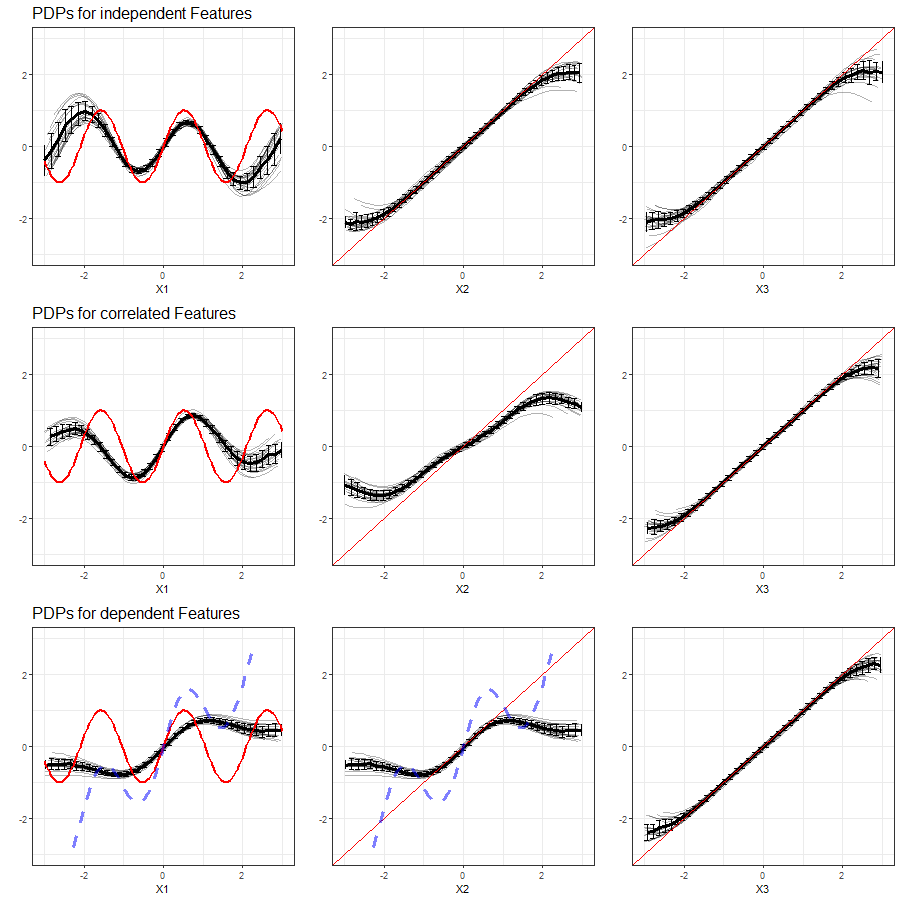
PDPs for features $x_1$, $x_2$ and $x_3$ (left to right) in Setting 2, based on multiple simulations with SVM as learning algorithm. Top row shows independent case, second row the correlated case and bottom row the dependent case. The red line represents the true effect of the respective feature on $y$, the blue dashed line is the true commmon effect of $x_1$ and $x_2$.

FIGURE 3.18: PDPs for features $x_1$, $x_2$ and $x_3$ (left to right) in Setting 2, based on multiple simulations with SVM as learning algorithm. Top row shows independent case, second row the correlated case and bottom row the dependent case. The red line represents the true effect of the respective feature on $y$, the blue dashed line is the true commmon effect of $x_1$ and $x_2$.

The findings derived from PDPs based on Random Forest are equivalently applicable to Support Vector Machines as machine learning algorithm. In the event of independent features, the PDPs can fairly well reveal the true feature effects, despite in the margins of the feature distrubutions. With strongly correlated or even dependent features, this ability vanishes and the PDPs of the affected features transform towards the variables' common effect.

3.3.4 Simulation of Setting 3: Missing informative feature $x_3$

In simulation setting 3, we assume that there are three variables with an impact on the data generating process of $y$. In the training process of the machine learning model, only two of those are considered. Consequently, when looking at the PDPs, we only compare the independent, the correlated and the dependent case for $x_1$ and $x_2$ respectively.

3.3.4.1 PDPs based on Linear Model

The results of our simulations in setting 3 based on the Linear Model are shown in figure 3.19: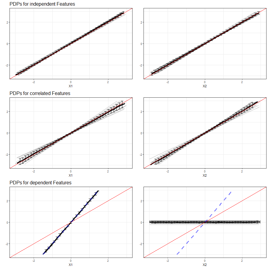

PDPs for features $x_1$ (left) and $x_2$ (right) in Setting 3, based on multiple simulations with LM as learning algorithm. Top row shows independent case, second row the correlated case and bottom row the dependent case. The red line represents the true effect of the respective feature on $y$, the blue dashed line is the true commmon effect of $x_1$ and $x_2$.

FIGURE 3.19: PDPs for features $x_1$ (left) and $x_2$ (right) in Setting 3, based on multiple simulations with LM as learning algorithm. Top row shows independent case, second row the correlated case and bottom row the dependent case. The red line represents the true effect of the respective feature on $y$, the blue dashed line is the true commmon effect of $x_1$ and $x_2$.

Compared to the PDPs of independent features the Linear Model produced in setting (3.10), the variation in individual PDPs is slightly higher with missing information from $x_3$. Overall, the learner can adequately reflect the linear feature effects of $x_1$ and $x_2$.
The increase in variablility between the individual PDPs is even more evident in the correlated case. On average, we still obtain the true linear effect of the correlated features, but there are some individual curves which do indicate a steeper or more moderate slope.
The PDPs drawn on basis of the Linear Model and dependent features indicate that for both individual features, the PDP consistently provides false effects on the predicted outcome. While both effects are actually linear with a slope of 1, the PDP for $x_1$ shows a steeper increase and $x_2$ fails completely. Nonetheless, the PDP for $x_1$ does reflect the common effect of both variables together.

3.3.4.2 PDPs based on Random Forest

The results of our simulations in setting 3 based on Random Forest are shown in figure 3.20: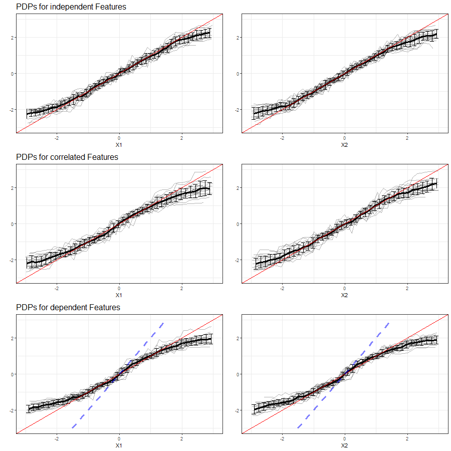

PDPs for features $x_1$ (left) and $x_2$ (right) in Setting 3, based on multiple simulations with RF as learning algorithm. Top row shows independent case, second row the correlated case and bottom row the dependent case. The red line represents the true effect of the respective feature on $y$, the blue dashed line is the true commmon effect of $x_1$ and $x_2$.

FIGURE 3.20: PDPs for features $x_1$ (left) and $x_2$ (right) in Setting 3, based on multiple simulations with RF as learning algorithm. Top row shows independent case, second row the correlated case and bottom row the dependent case. The red line represents the true effect of the respective feature on $y$, the blue dashed line is the true commmon effect of $x_1$ and $x_2$.

Compared to setting (3.10), where all relevant feature variables were taken into account for the training of the model, the variation in PDP curves in setting (3.12) is larger. Between features $x_1$ and $x_2$, which are independent, there is no systematic difference traceable from the PDPs.
Other than an increased variability between the individual PDP curves and a slightly tighter prediction interval, with correlated features and Random Forest as learner, there is no apparent deviation to the PDPs of independent features.
In accordance with the observations made in setting (3.10), the interval of predicted values for dependent features become even smaller while the PDP curves further deviate from the true effect. Neither the individual effect of each feature, nor their common effect are illustrated adequately.

3.3.4.3 PDPs based on Support Vector Machines

The results of our simulations in setting 3 based on Support Vector Machines are shown in figure 3.21: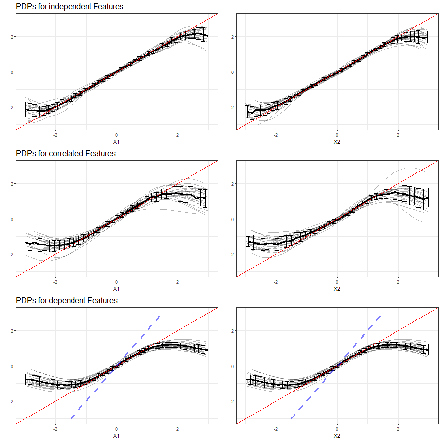

PDPs for features $x_1$ (left) and $x_2$ (right) in Setting 3, based on multiple simulations with SVM as learning algorithm. Top row shows independent case, second row the correlated case and bottom row the dependent case. The red line represents the true effect of the respective feature on $y$, the blue dashed line is the true commmon effect of $x_1$ and $x_2$.

FIGURE 3.21: PDPs for features $x_1$ (left) and $x_2$ (right) in Setting 3, based on multiple simulations with SVM as learning algorithm. Top row shows independent case, second row the correlated case and bottom row the dependent case. The red line represents the true effect of the respective feature on $y$, the blue dashed line is the true commmon effect of $x_1$ and $x_2$.

Similar to learning based on Random Forest, the SVM learner with missing feature variable $x_3$ produces a higher variability between the simulated PDP curves. The margin areas, where the PDPs cannot adequately reflect the linear dependence, are broader than in setting (3.10).
In the event of the two remaining features $x_1$ and $x_2$ being strongly correlated, the issue of larger variability between the individual simulations aggravates and the ability to reveal the linear effect ceases.
With a perfect multicollinearity of $x_1$ and $x_2$, the variablity of the individual PDP curves becomes smaller, but at the same time the models' ability to uncover the true linear effect vanishes. The interval of predicted values is remarkably smaller than in the independent case.

3.3.5 Simulation Settings: Categorical Features

In this chapter we want to investigate the impact of dependencies between two categorical and between a categorical and a numerical feature. For this purpose, we simulate data with a number of 1000 randomly drawn observations and three feature variables, where:

$x_1$ categorical variable $\in \{0,1\}$,
$x_2$ categorical variable $\in \{A,B,C\}$,
$x_3$ numerical variable with $x_3 \sim N(\mu, \sigma^2)$.

All features are characterized by their linear relationship with the target variable: $y=x_1+x_2+x_3+\varepsilon$.

Again, in order to isolate the individual effects of two dependent features on their respective PDPs, we define three different simulation settings:

1. Independent Case: In this setting, the feature variables are drawn independently from each other, i.e. the observations are randomly sampled with the following parameters:

$x_1: P(x_1=1)=P(x_1=0)=0.5$
$x_2: P(x_2=A)=0.475, P(x_2=B)=0.175, P(x_2=C)=0.35$
$x_3: P(x_3 \sim N(1,1))=0.5, P(x_3 \sim N(20,2))=0.5$

The association between $x_1$ and $x_2$ can be measured by the corrected contingency coefficient, which is rather low with a value of 0.10. In accordance with the approach in chapter 3.2.3, we calculate the association between $x_1$ and $x_3$ by means of the variance-explained measure. With a value of 0.01 we take the independence assumption as confirmed.

2. Dependency between two categorical features: In this setting, $x_1$ and $x_2$ are depending on each each other, i.e. the observations are randomly sampled with the following parameters:

$x_1: P(x_1=1)=P(x_1=0)=0.5$
$x_2: \begin{cases} P(x_2=A)=0.90, P(x_2=B)=0.10, P(x_2=C)=0), \text{if } x_1=0, \\ P(x_2=A)=0.05, P(x_2=B)=0.25, P(x_2=C)=0.70), \text{if } x_1=1 \end{cases}$
$x_3: P(x_3 \sim N(1,1))=0.5, P(x_3 \sim N(20,2))=0.5$

The corrected contingency coefficient of 0.94 comfirms a strong association between features $x_1$ and $x_2$.

3. Dependency between categorical and numerical features: In this setting, $x_1$ and $x_3$ are depending on each each other, i.e. the observations are randomly sampled with the following parameters:

$x_1: P(x_1=1)=P(x_1=0)=0.5$
$x_2: P(x_2=A)=0.475, P(x_2=B)=0.175, P(x_2=C)=0.35$
$x_3: \begin{cases} x_3 \sim N(1,1), \text{if } x_1=0 \\ x_3 \sim N(20,2), \text{if } x_1=1 \end{cases}$

With a value of 0.986, the variance-explained measure indicates a substantial degree of dependency between $x_1$ and $x_3$.

3.3.5.1 PDPs based on Linear Model

Figure 3.22 shows the PDPs for all feature variables and all simulation settings based on the Linear Model.

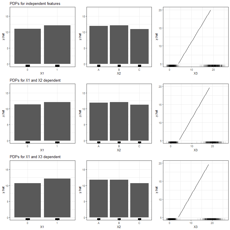
PDPs for categorical features $x_1$, $x_2$ and numerical feature $x_3$ (left to right), based on simulated data and LM as learning algorithm. Top row shows independent case, second row the case of two dependent categorical features and the bottom row the case of a numerical feature depending on a categorical feature.

FIGURE 3.22: PDPs for categorical features $x_1$, $x_2$ and numerical feature $x_3$ (left to right), based on simulated data and LM as learning algorithm. Top row shows independent case, second row the case of two dependent categorical features and the bottom row the case of a numerical feature depending on a categorical feature.

Apparently, the Linear Model is robust against our simulated dependencies, since the PDPs of the correlated and dependent features do not differ significantly from those of independent features.

3.3.5.2 PDPs based on Random Forest

Figure 3.23 shows the PDPs for all feature variables and all simulation settings based on Random Forest.

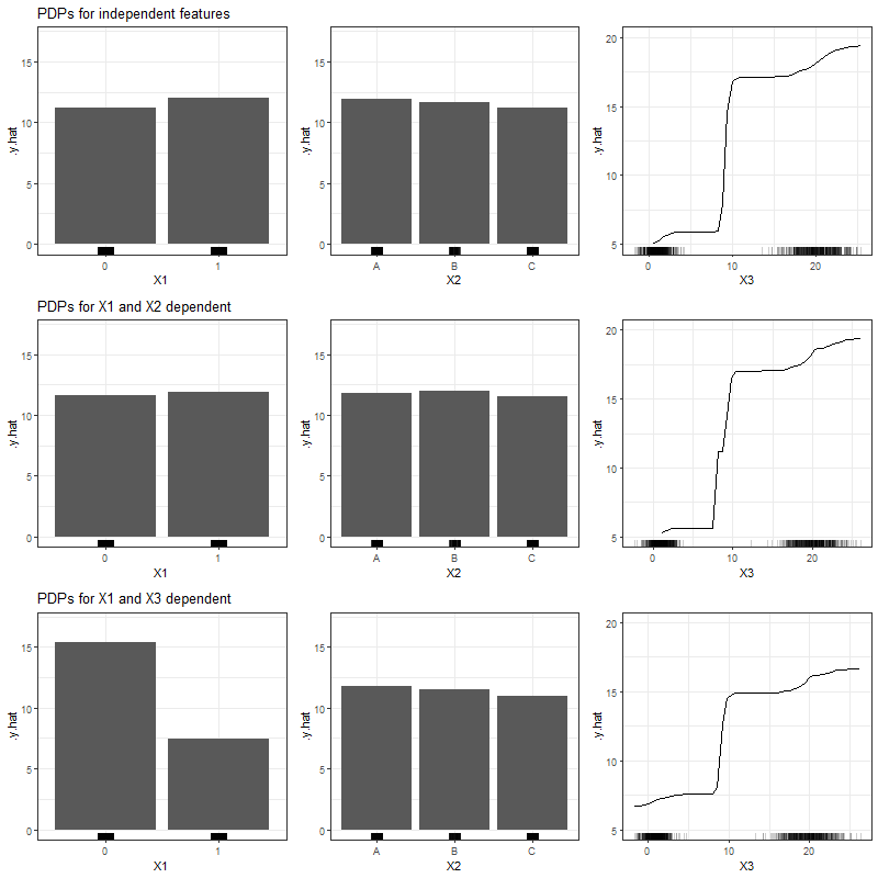
PDPs for categorical features $x_1$, $x_2$ and numerical feature $x_3$ (left to right), based on simulated data and RF as learning algorithm. Top row shows independent case, second row the case of two dependent categorical features and the bottom row the case of a numerical feature depending on a categorical feature.

FIGURE 3.23: PDPs for categorical features $x_1$, $x_2$ and numerical feature $x_3$ (left to right), based on simulated data and RF as learning algorithm. Top row shows independent case, second row the case of two dependent categorical features and the bottom row the case of a numerical feature depending on a categorical feature.

Based on Random Forest, the partial dependence function seems to be impacted much stronger by our simulated dependencies, since the PDPs for dependent variables indicate feature effects which differ from those in the independent case. This is particularly true for a strong association between a categorical an a numerical variable (bottom row of figure 3.23).

3.3.5.3 PDPs based on Support Vector Machines

Figure 3.24 shows the PDPs for all feature variables and all simulation settings based on Support Vector Machines.

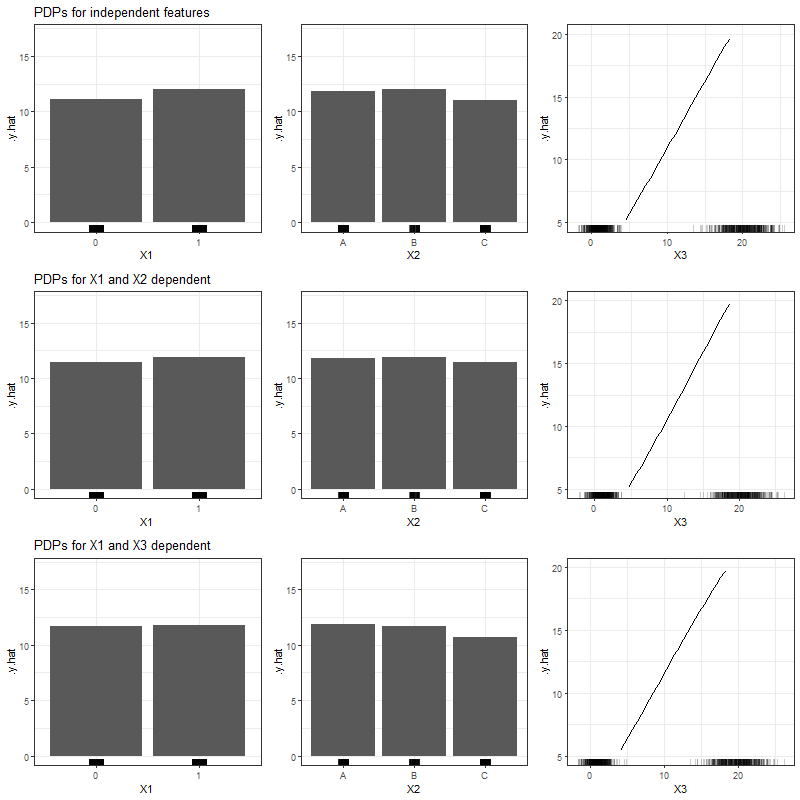
FIGURE 3.24: PDPs for categorical features $x_1$, $x_2$ and numerical feature $x_3$ (left to right), based on simulated data and RF as learning algorithm. Top row shows independent case, second row the case of two dependent categorical features and the bottom row the case of a numerical feature depending on a categorical feature.

In accordancy with our findings based on the Linear Model, the predicted effects based on SVM seem to be robust against our simulated dependencies, since the PDPs for the individual settings do not differ significantly from the independent case.

3.4 Extrapolation Problem: Simulation

3.4.1 Simulation based on established learners

In the problem description of this chapter we announced that, in addition to the issue with dependent features, we want to investigate the extrapolation problem and its implications for the computation of partial dependence plots. For this purpose, we use the dataset introduced in chapter 3.1, which was simulated once with $x_1$ and $x_2$ independent, and once with both features strongly correlated. Remember that in a next step, the observed data was manipulated by cutting out all observations with $x_1 \in [0, 1.5] \wedge x_2 \in [0, 1.5]$, and thus artificially producing an area with no observations (see figure 3.2).

Now we are looking at the PDPs resulting from these modifications. Figure 3.25 compares the PDP curves derived for both features based on the complete, uncorrelated dataset to its manipulated version with missing values.

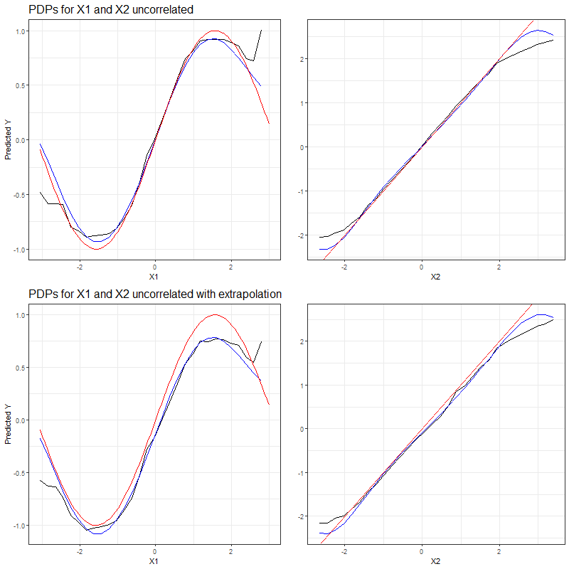
PDPs for uncorrelated features $x_1$ (left) and $x_2$ (right) based on complete simulated dataset (top row) and based on manipulated dataset with missing observations (bottom row). The red curve represents the true effect of the feature for which the PDP is drawn, while the PDPs derived from the machine learning models are represented by curves drawn in black (Random Forest) and blue (SVM).

FIGURE 3.25: PDPs for uncorrelated features $x_1$ (left) and $x_2$ (right) based on complete simulated dataset (top row) and based on manipulated dataset with missing observations (bottom row). The red curve represents the true effect of the feature for which the PDP is drawn, while the PDPs derived from the machine learning models are represented by curves drawn in black (Random Forest) and blue (SVM).

The first row of PDPs in figure 3.25, computed on basis of the complete dataset of uncorrelated features, adequately reflects the true effects of $x_1$ and $x_2$ (red curves). In the presence of an extrapolation problem, the adequacy of the predicted effects decreases. Especially with the more complex, nonlinear effect of $x_1$, extrapolation causes a clearly visible deviation between the partial dependence curves and the true feature effect, irrespective of the learner.

In figure 3.26 we do the same comparison, but this time based on the dataset with strongly correlated features.

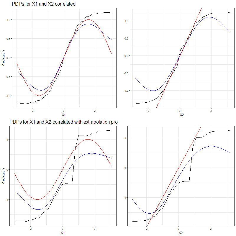
PDPs for correlated features $x_1$ (left) and $x_2$ (right) based on complete simulated dataset (top row) and based on manipulated dataset with missing observations (bottom row). The red curve represents the true effect of the feature for which the PDP is drawn, while the PDPs derived from the machine learning models are represented by curves drawn in black (Random Forest) and blue (SVM).

FIGURE 3.26: PDPs for correlated features $x_1$ (left) and $x_2$ (right) based on complete simulated dataset (top row) and based on manipulated dataset with missing observations (bottom row). The red curve represents the true effect of the feature for which the PDP is drawn, while the PDPs derived from the machine learning models are represented by curves drawn in black (Random Forest) and blue (SVM).

From the first row of PDPs in figure 3.26, we again discover the difficulty to obtain reliable PDPs when features are dependent. The results in the bottom row of figure 3.26 are even more striking: with a combination of dependent features and extrapolation, the PDPs come up with estimated effects which are far from the true effects on the prediction. Those deviations seem to occur irrespective of the learning algorithm.

3.4.2 Simulation based on own prediction function

So far, all our analyses were based on the established learning algorithms LM, RF and SVM. We have seen that the choice of the learner does have an impact on the suitability of PDP curves. Obviously there is a countless number of other possibilities to come up with prediction functions other than the ones we have seen. PDPs are prone to fail when this prediction function is doing 'weird' stuff in areas outside the feature distribution. This can happen due to the fact that the learner minimizes the loss based on training data while there is no penalization for extrapolation (Molnar 2019).

Let's illustrate the issue with an example. Assume we want to predict the size of a potato ($\hat{y}$) by means of the share of maximum amount of soil ($x_1$) and the share of maximum amount of water ($x_2$) available during the process of growing the plant. The feature variables are dependent in the sense that when using a larger amount of soil, the farmer would also use a larger amount of water, i.e. $x_1$ and $x_2$ are positively correlated. Typically, the more ressources the farmer invests, the larger the crops. The corresponding model is basically a simple linear regression which adds up the two components.

In the event of improper planting, meaning the usage of a too large amount of water in proportion to the soil (and vice versa), the plant would die and the result would be a potato of size 0. This is exactly what our self-constructed prediction function predicts. Luckily, all farmers in our dataset know how to grow potatoes, therefore there are no such zero cases in the underlying observations. Figure 3.27 illustrates our observations as points and the prediction function as shaded background colour.

Visualization of the observed data points (n=100) and the self-contructed prediction function. Dark blue background colour indicates a predicted potato size of zero which increases with the brightness of the yellow shaded background colour.

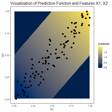
FIGURE 3.27: Visualization of the observed data points (n=100) and the self-contructed prediction function. Dark blue background colour indicates a predicted potato size of zero which increases with the brightness of the yellow shaded background colour.

In view of the observed data, one would expect to uncover a linear effect of both feature variables when looking at the corresponding PDPs. As we can see in figure 3.28, this is not necessarily the case. While the two-dimensional PDP perfectly depicts the prediction function, the individual PDPs for feature $x_1$ and $x_2$ fail in the areas where the prediction function does 'weird' stuff compared to what has been observed.

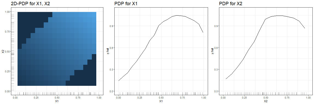
The first plot shows the two-dimensional PDP for features $x_1$ and $x_2$. The darker the background colour, the smaller the predicted values. The other plots are the PDPs derived for feature $x_1$ and $x_2$ respectively. Up to a value of approximately 0.5 both partial dependence curves are mostly linear and bend at larger $x_1$- / $x_2$-values.

FIGURE 3.28: The first plot shows the two-dimensional PDP for features $x_1$ and $x_2$. The darker the background colour, the smaller the predicted values. The other plots are the PDPs derived for feature $x_1$ and $x_2$ respectively. Up to a value of approximately 0.5 both partial dependence curves are mostly linear and bend at larger $x_1$- / $x_2$-values.

3.5 Summary

Our analysis of partial dependence plots in the context of dependent features and missing values has revealed that both a violation of the underlying independence assumption and the presence of areas with no observations can have a significant impact on the marginalized feature effects. As a consequence, there is a risk of misinterpretation of the effect of features in $x_S$. Hooker and Mentch (2019) propose to make use of local explanation methods in order to avoid extrapolation. ICE plots, as an example, can be restricted to values in line with the distribution of observed data. However, the authors also point out that this approach cannot serve as a global representation of the learned model (Hooker and Mentch 2019).

In our simulations, we have also seen cases where the PDP (or the underlying machine learning algorithm) proved to be relatively robust against the dependency of features. Further to the independence assumtion, there are also other parameters playing a role for the accuracy of PDPs, like the grid size, the number of observations, the learning algorithm, variance in the data, complexity of the data generating process, etc.

In practical applications it is recommended to analyse the variables used in the model, both by means of correlation and/or association measures and content-wise in liason with experts having domain knowledge. Furthermore, data scientists can apply methods based on the conditional expectation, such as M-plots or ALE plots. The concept and limitations of the latter will be discussed in chapters 6-8 of this book.

References

Fahrmeir, L., C. Heumann, R. Künstler, I. Pigeot, and G. Tutz. 2016. Statistik: Der Weg Zur Datenanalyse. Springer-Lehrbuch. Springer Berlin Heidelberg. https://books.google.de/books?id=rKveDAAAQBAJ.

Fahrmeir, L., T. Kneib, S. Lang, and B. Marx. 2013. Regression: Models, Methods and Applications. Springer Berlin Heidelberg. https://books.google.de/books?id=EQxU9iJtipAC.

Fanaee-T, Hadi, and Joao Gama. 2013. “Event Labeling Combining Ensemble Detectors and Background Knowledge.” Progress in Artificial Intelligence. Springer Berlin Heidelberg, 1–15. doi:10.1007/s13748-013-0040-3.

Goldstein, Alex, Adam Kapelner, Justin Bleich, and Emil Pitkin. 2013. “Peeking Inside the Black Box: Visualizing Statistical Learning with Plots of Individual Conditional Expectation.” Journal of Computational and Graphical Statistics 24 (September). doi:10.1080/10618600.2014.907095.

Hastie, T., R. Tibshirani, and J. Friedman. 2013. The Elements of Statistical Learning: Data Mining, Inference, and Prediction. Springer Series in Statistics. Springer New York. https://books.google.de/books?id=yPfZBwAAQBAJ.

Hooker, Giles, and Lucas Mentch. 2019. “Please Stop Permuting Features: An Explanation and Alternatives.” arXiv E-Prints, May, arXiv:1905.03151.

Molnar, Christoph. 2019. Interpretable Machine Learning: A Guide for Making Black Box Models Explainable.

Limitations of Interpretable Machine Learning Methods