Chapter 4 Recurrent neural networks and their applications in NLP

Author: Marianna Plesiak

Supervisor: Christian Heumann

4.1 Structure and Training of Simple RNNs

Recurrent neural networks (RNNs) enable to relax the condition of non-cyclical connections in the classical feedforward neural networks which were described in the previous chapter. This means, while simple multilayer perceptrons can only map from input to output vectors, RNNs allow the entire history of previous inputs to influence the network output. (Graves 2013)

The first part of this chapter provides the structure definition of RNNs, presents the principles of their training and explains problems with backpropagation. The second part covers gated units, an improved way to calculate hidden states. The third part gives an overview of some extended versions of RNNs and their applications in NLP.

4.1.1 Network Structure and Forwardpropagation

An unfolded computational graph can visualize the repetitive structure of RNNs:

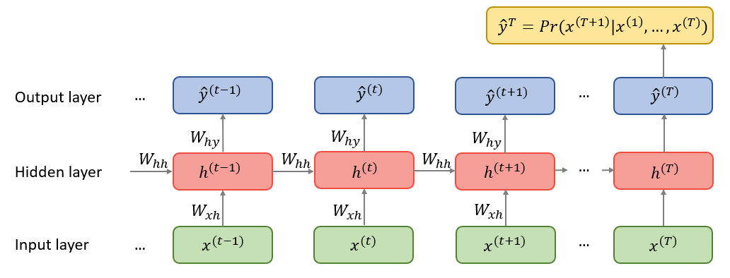
FIGURE 4.1: Unfolded computatinal graph of an RNN. Source: Own figure.

Each node is associated with a network layer at a particular time instance. Inputs \(x^{(t)}\) must be encoded as numeric vectors, for instance word embeddings or one-hot encoded vectors, see the previous chapter. Recurrently connected vectors \(h\) are called hidden states and represent the outputs of the hidden layer. At time \(t\), a hidden state \(h^{(t)}\) combines information from the previous hidden state \(h^{(t-1)}\) as well as the new input \(x^{(t)}\) and transmits it to the next hidden state. Obviously, such an architecture requires the initialization of \(h^{(0)}\) since there is no memory at the very beginning of the sequence processing. Given the hidden sequences, output vectors \(\hat{y}^{(t)}\) are used to build the predictive distribution \(Pr(x^{(t+1)}|y^{(t)})\) for the next input (Graves 2013). Since the predictions are created at each time instance \(t\), the total output has a shape \([\#\ time\_steps, \#\ output\_features]\). However, in some cases the whole history of output features is not necessary. For example, in sentiment analysis the last output of the loop is sufficient because it contains the entire information about the sequence. (Chollet 2018)

The unfolded recurrence can be formalized as following:

After \(t\) steps, the function \(g^{(t)}\) takes into account the whole sequence \((x^{(t)},x^{(t-1)},...,x^{(2)}, x^{(1)})\) and produces the hidden state \(h^{(t)}\). Because of its cyclical structure, \(g^{(t)}\) can be factorized into the repeated application of the same function \(f\). This function can be considered to be a universal model with parameters \(\theta\) which are shared across all time steps and generalized for all sequence lengths. This concept is called parameter sharing and is illustrated in the unfolded computational graph as a reuse of the same matrices \(W_{xh}\), \(W_{hh}\) and \(W_{hy}\) through the entire network. (Goodfellow, Bengio, and Courville 2016)

Considering a recurrent neural network with one hidden layer that is used to predict words or characters, the output should be discrete and the model maps input sequence to output sequence of the same length. Then, the forward propagation is computed by iterating the following equations:

where, according to Graves (2013), the parameters and functions denote the following:

• \(x^{(t)}\), \(h^{(t)}\) and \(y^{(t)}\): input, hidden state and output at time step \(t\) respectively;
• \(\mathcal{f}\): activation function of the hidden layer. Usually it is a saturating nonlinear function such as a sigmoid activation function ( Sutskever, Vinyals, and Le (2014) and Mikolov et al. (2010));
• \(W_{hh}\): weight matrix connecting recurrent connections between hidden states;
• \(W_{xh}\): weight matrix connecting inputs to a hidden layer;
• \(W_{hy}\): weight matrix connecting hidden states to outputs;
• \(\mathcal{s}\): output layer function. If the model is used to predict words, the softmax function is usually chosen as it returns valid probabilities over the possible outputs (Mikolov et al. 2010);
• \(a\), \(b\): input and output bias vectors.

Since inputs \(x^{(t)}\) are usually encoded as one-hot-vectors, the dimension of a vector representing one word corresponds to the size of vocabulary. The size of a hidden layer must reflect the size of training data. The model training requires initialization of the initial state \(h^{(0)}\) as well as the weight matrices, which are usually set to small random values (Mikolov et al. 2010). Since the model is used to compute the predictive distributions \(Pr(x^{(t+1)}|y^{(t)})\) at each time instance \(t\), the network distribution is denoted as following:

and the total loss \(\mathcal{L(x)}\), which must be minimized during the training, is simply the sum of losses over all time steps denoted as the negative log-likelihood of \(Pr(x)\):

(Graves 2013)

4.1.2 Backpropagation

To train the model, one must calculate the gradients for the three weight matrices \(W_{xh}\), \(W_{hh}\) and \(W_{hy}\). The algorithm differs from a regular backpropagation because a chain rule must be applied recursively, and the gradients are summed up through the network (Boden 2002). Using the notation \(\mathcal{L^{(t)}}\) as the output at time \(t\), one must first estimate single losses at each time step and then sum them up in order to obtain total loss \(\mathcal{L(x)}\).

Chen (2016) provides a nice guide to backpropagation for a simple RNN in the meaning of equations (??) and (??). According to him, the gradient w.r.t. \(W_{hy}\) for a single time step \(t\) is calculated as follows:

Since \(W_{hy}\) is shared across all time sequence, the total loss w.r.t. the weight matrix connecting hidden states to outputs is simply a sum of single losses:

Similarly, derivation of the gradient w.r.t. \(W_{hh}\) for a single time step is obtained as follows:

However, the last part \(h^{(t)}\) also depends on \(h^{(t-1)}\) and the gradient can be rewritten according to the Backpropagation Through Time algorithm (BPTT) starting from \(t\) and going back to the initial hidden state at time step \(k=0\):

Single gradients are again aggregated to yield the overall loss w.r.t \(W_{hh}\):

The derivation of gradients w.r.t. \(W_{xh}\) is similar to those w.r.t \(W_{hh}\) because both \(h^{(t-1)}\) and \(x^{(t)}\) contribute to \(h^{(t)}\) at time step \(t\). The derivative w.r.t. \(W_{xh}\) for the whole sequence is then obtained by summing up all contributions from \(t\) to \(0\) via backpropagation for all time steps:

The derivatives w.r.t. the bias vectors \(a\) and \(b\) are calculated based on the same principles and thus are not shown here explicitly.

4.1.3 Vanishing and Exploding Gradients

In order to better understand the mathematical challenges of BPTT, one should consider equation (??), and in particular the factor \(\frac{\partial h^{(t)}}{\partial h^{(k)}}\). Pascanu, Mikolov, and Bengio (2013) go into detail and show that it is a chain rule in itself and can be rewritten as a product \(\frac{\partial h^{(t)}}{\partial h^{(t-1)}} \frac{\partial h^{(t-1)}}{\partial h^{(t-2)}} \ldots \frac{\partial h^{(2)}}{\partial h^{(1)}}\). Since one computes the derivative of a vector w.r.t another vector, the result will be a product of \(t-k\) Jacobian matrices whose elements are the pointwise derivatives:

Thus, with small values in \(W_{hh}\) and many matrix multiplications the norm of the gradient shrinks to zero exponentially fast with \(t-k\) which results in a vanishing gradient problem and the loss of long term contributions. Exploding gradients refer to the opposite behaviour when the norm of the gradient increases largely and leads to a crash of the model. Pascanu, Mikolov, and Bengio (2013) give an overview of techniques for dealing with the exploding and vanishing gradients. Among other solutions they mention proper initialisation of weight matrices, sampling \(W_{hh}\) and \(W_{xh}\) instead of learning them, rescaling or clipping the gradient’s components (putting a maximum limit on it) or using L1 or L2 penalties on the recurrent weights. Even more popular models are gated RNNs which explicitly address the vanishing gradients problem and will be explained in the next subchapter.

4.2 Gated RNNs

Main feature of gated RNNs is the ability to store long-term memory for a long time and at the same time to account for new inputs as effectively as possible. In modern NLP, two types of gated RNNs are used widely: Long Short-Term Memory networks and Gated Recurrent Units.

4.2.1 LSTM

Long Short-Term Memory (LSTM) networks were introduced by Hochreiter and Schmidhuber (1997) with the purpose of dealing with problems of long term dependencies. Figure 4.2 illustrates the complex architecture of LSTM hidden state. Instead of a simple hidden unit that combines inputs and previous hidden states linearly and outputs their nonlinear transformation to the next step, hidden units are now extended by special input, forget and output gates that help to control the flow of information. Such more complex units are called memory cells, and the following equations show how a LSTM uses the gating mechanism to calculate the hidden state within a memory cell:

First, the forget gate \(f^{(t)}\) decides which values of the previous output \(h^{(t-1)}\) to forget. The next step involves deciding which information will be stored in the internal cell state \(c^{(t)}\). This step consists of the following two parts: 1) the old cell state \(c^{(t-1)}\) is multiplied by \(f^{(t)}\) in order to forget information; 2) new candidates are calculated in \(g^{(t)}\) and multiplied by the input gate \(i^{(t)}\) in order to add new information. Finally, the output \(h^{(t)}\) is produced with help of the output gate \(o^{(t)}\) and applying a \(tanh\) function to the cell state in order to only output selected values. (Goodfellow, Bengio, and Courville (2016), Graves (2013))

4.2.2 GRU

In 2014, Cho et al. (2014) introduced Gated Recurrent Units (GRU) whose structure is simpler than that of LSTM because they have only two gates, namely reset and update gate. The hidden state is thus calculated as follows:

First, the reset gate \(r^{(t)}\) decides how much the previous hidden state \(h^{(t-1)}\) is ignored, so if \(r^{(t)}\) is close to \(0\), the hidden state is forced to drop past irrelevant information and reset with current input \(x^{(t)}\). A candidate hidden state \(\tilde{h}^{(t)}\) is then obtained in the following three steps: 1) weight matrix \(W_{xh}\) is multiplied by current input \(x^{(t)}\); 2) weight matrix \(W_{hh}\) is multiplied by the element-wise product (denoted as \(\odot\)) of reset gate \(r^{(t)}\) and previous hidden state \(h^{(t)}\); 3) both products are added and a \(tanh\) function is applied in order to output the candidate values for a hidden state. On the other hand, the update gate \(z^{(t)}\) decides how much of the previous information stored in \(h^{(t-1)}\) will carry over to \(h^{(t)}\) and how much the new hidden state must be updated with the candidate \(\tilde{h}^{(t)}\). Thus, the update gate combines the functionality of LSTM forget and input gates and helps to capture long-term memory. Cho et al. (2014) used the GRU in the machine translation task and showed that the novel hidden units can achieve good results in term of BLEU score (see chapter 11 for definition) while being computationally cheaper than LSTM.

Figure 4.2 visualizes the architecture of hidden states of gated RNNs mentioned above and illustrates their differences:

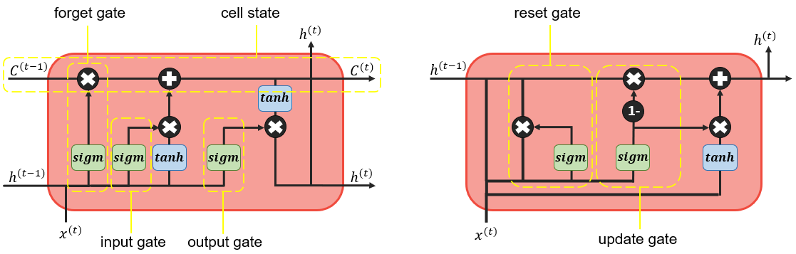
FIGURE 4.2: Structure of a hidden unit. LSTM on the right and GRU on the left. Source: Own figure inspired by http://colah.github.io/posts/2015-08-Understanding-LSTMs/

4.3 Extensions of Simple RNNs

In most challenging NLP tasks, such as machine translation or text generation, one-layer RNNs even with gated hidden states cannot often deliver successful results. Therefore more complicated architectures are necessary. Deep RNNs with several hidden layers may improve model performance significantly. On the other hand, completely new designs such as Encoder-Decoder architectures are most effective when it comes to mapping sequences of an arbitrary length to a sequence of another arbitrary length.

4.3.1 Deep RNNs

The figure 4.1 shows that each layer is associated with one parameter matrix so that the model is considered shallow. This structure can be extended to a deep RNN, although the depth of an RNN is not a trivial concept since its units are already expressed as a nonlinear function of multiple previous units.

4.3.1.1 Stacked RNNs

In their paper Graves, Mohamed, and Hinton (2013) use a deep RNN for speech recognition where the depth is defined as stacking \(N\) hidden layers on top of each other with \(N>1\). In this case the hidden vectors are computed iteratively for all hidden layers \(n=1\) to \(N\) and for all time instances \(t=1\) to \(T\):

As a hidden layer function Graves, Mohamed, and Hinton (2013) choose bidirectional LSTM. Compared to regular LSTM, BiLSTM can train on inputs in their original as well as reversed order. The idea is to stack two separate hidden layers one on another while one of the layers is responsible for the forward information flow and another one for the backward information flow. Especially in speech recognition one must take in consideration future context, too, because pronouncement depends both on previous and next phonemes. Thus, BiLSTMs are able to access long-time dependencies in both input directions. Finally, Graves, Mohamed, and Hinton (2013) compare different deep BiLSTM models (from 1 to 5 hidden layers) with unidirectional LSTMs and a pre-trained RNN transducer (BiLSTM with 3 hidden layers pretrained to predict each phoneme given the previous ones) and show clear advantage of deep networks over shallow designs.

4.3.1.2 Deep Transition RNNs

Pascanu et al. (2013) proposed another way to make an RNN deeper by introducing transitions, one or more intermediate nonlinear layers between input to hidden, hidden to output or two consecutive hidden states. They argue that extending input-to-hidden functions helps to better capture temporal structure between successive inputs. A deeper hidden-to-output function, DO-RNN, can make hidden states more compact and therefore enables the model to summarize the previous inputs more efficiently. A deep hidden-to-hidden composition, DT-RNN, allows for the hidden states to effectively add new information to the accumulated summaries from the previous steps. They note though, because of including deep transitions, the distances between two variables at \(t\) and \(t+1\) become longer and the problem of loosing long-time dependencies may occur. One can add shortcut connections to provide shorter paths for gradients, such networks are referred to as DT(S)-RNNs. If deep transitions with shortcuts are implemented both in hidden and output layers, the resulting model is called DOT(S)-RNNs. Pascanu et al. (2013) evaluate these designs on the tasks of polyphonic music prediction and character- or word-level language modelling. Their results reveal that deep transition RNNs clearly outperform shallow RNNs in terms of perplexity (see chapter 11 for definition) and negative log-likelihood.

4.3.2 Encoder-Decoder Architecture

4.3.2.1 Design and Training

The problem of mapping variable-length input sequences to variable-length output sequences is known as Sequence-to-Sequence or seq2seq learning in NLP. Although originally applied in machine translation tasks (Sutskever, Vinyals, and Le (2014), Cho et al. (2014)), the seq2seq approach achieved state-of-the-art results also in speech recognition (Prabhavalkar et al. 2017) and video captioning (Venugopalan et al. 2015). According to Cho et al. (2014), the seq2seq model is composed of two parts as illustrated below:

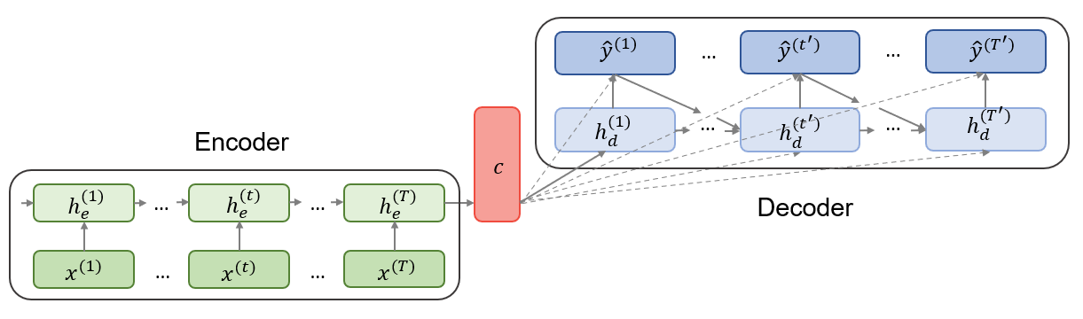
FIGURE 4.3: Encoder-Decoder architecture. Source: Own figure based on Cho et al. (2014).

The first part is an encoder, an RNN which is trained on input sequences in order to obtain a large summary vector \(c\) with a fixed dimension. This vector is called context and is usually a simple function of the last hidden state. Sutskever, Vinyals, and Le (2014) used the final encoder hidden state as context such that \(c=h_{e}^{(T)}\). The second part of the model is a decoder, another RNN which generates predictions given the context \(c\) and all the previous outputs. In contrast to a simple RNN described at the beginning of this chapter, decoder hidden states \(h_{d}^{(t)}\) are now conditioned on the previous outputs \(y^{(t)}\), previous hidden states \(h_{d}^{(t)}\) and the summary vector \(c\) from the encoder part. Therefore, the conditional distribution of the one-step prediction is obtained by:

Both parts are trained simultaneously to maximize the conditional log-likelihood \(\frac{1}{N}\sum_{n=1}^{N}\log{p_{\theta}(y_{n}|x_{n})}\), where \(\theta\) denotes the set of model parameters and \((y_{n},x_{n})\) is an (input sequence, output sequence) pair from the training set with size \(N\) (Cho et al. (2014)).

4.3.2.2 Multi-task seq2seq Learning

Luong et al. (2015) extended the idea of encoder-decoder architecture even further by allowing multi-task learning (MLT) for seq2seq models. MLT aims to improve performance of one task using other related tasks such that one task complements another. In their paper, they investigate the following three settings: a) one-to-many - where the encoder is shared between different tasks such as translation and syntactic parsing, b) many-to-one - where the encoders learn different tasks such as translation and image captioning and the decoder is shared, c) many-to-many - where the model consists of multiple encoders and decoders which is the case of autoencoders, an unsupervised task used to learn a representation of monolingual data.

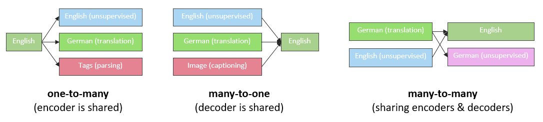
FIGURE 4.4: Multi-task settings. Source: Luong et al. (2015).

Luong et al. (2015) consider German-to-English and English-to-German translations as the primary task and try to determine whether other tasks can improve their performance and vice versa. After training deep LSTM models with four layers for different task combinations, they conclude that MLT can improve the performance of seq2seq models substantially. For instance, the translation quality improves after adding a small number of parsing minibatches (one-to-many setting) or after the model have been trained to generate image captions (many-to-one setting). In turn, translation task helps to parse large data corpus much better (one-to-many setting). In contrast to these achievements, autoencoder task does not show significant improvements in translation after two unsupervised learning tasks on English and German language data.

4.4 Conclusion

RNNs are powerful models for sequential data. Even in their simple form they can show valid results in different NLP tasks but their shortcomings led to introduction of more flexible networks such as gated units and encoder-decoder designs described in this chapter. As NLP has become a highly discussed topic in the recent years, even more advanced concepts such as Transfer Learning and Attention have been introduced, which still base on an RNN or its extension. However, RNNs are not the only type of neural networks used in NLP. Convolutional neural networks also find their application in modern NLP, and the next chapter will describe them.

References

Boden, Mikael. 2002. “A Guide to Recurrent Neural Networks and Backpropagation.” The Dallas Project.

Chen, Gang. 2016. “A Gentle Tutorial of Recurrent Neural Network with Error Backpropagation.” arXiv Preprint arXiv:1610.02583.

Cho, Kyunghyun, Bart Van Merriënboer, Caglar Gulcehre, Dzmitry Bahdanau, Fethi Bougares, Holger Schwenk, and Yoshua Bengio. 2014. “Learning Phrase Representations Using Rnn Encoder-Decoder for Statistical Machine Translation.” arXiv Preprint arXiv:1406.1078.

Chollet, Francois. 2018. Deep Learning Mit Python Und Keras: Das Praxis-Handbuch Vom Entwickler Der Keras-Bibliothek. MITP-Verlags GmbH & Co. KG.

Goodfellow, Ian, Yoshua Bengio, and Aaron Courville. 2016. Deep Learning. MIT press.

Graves, Alex. 2013. “Generating Sequences with Recurrent Neural Networks.” arXiv Preprint arXiv:1308.0850.

Graves, Alex, Abdel-rahman Mohamed, and Geoffrey Hinton. 2013. “Speech Recognition with Deep Recurrent Neural Networks.” In 2013 Ieee International Conference on Acoustics, Speech and Signal Processing, 6645–9. IEEE.

Hochreiter, Sepp, and Jürgen Schmidhuber. 1997. “Long Short-Term Memory.” Neural Computation 9 (8). MIT Press: 1735–80.

Luong, Minh-Thang, Quoc V Le, Ilya Sutskever, Oriol Vinyals, and Lukasz Kaiser. 2015. “Multi-Task Sequence to Sequence Learning.” arXiv Preprint arXiv:1511.06114.

Mikolov, Tomáš, Martin Karafiát, Lukáš Burget, Jan Černocky, and Sanjeev Khudanpur. 2010. “Recurrent Neural Network Based Language Model.” In Eleventh Annual Conference of the International Speech Communication Association.

Pascanu, Razvan, Caglar Gulcehre, Kyunghyun Cho, and Yoshua Bengio. 2013. “How to Construct Deep Recurrent Neural Networks.” arXiv Preprint arXiv:1312.6026.

Pascanu, Razvan, Tomas Mikolov, and Yoshua Bengio. 2013. “On the Difficulty of Training Recurrent Neural Networks.” In International Conference on Machine Learning, 1310–8.

Prabhavalkar, Rohit, Kanishka Rao, Tara N Sainath, Bo Li, Leif Johnson, and Navdeep Jaitly. 2017. “A Comparison of Sequence-to-Sequence Models for Speech Recognition.” In Interspeech, 939–43.

Sutskever, Ilya, Oriol Vinyals, and Quoc V Le. 2014. “Sequence to Sequence Learning with Neural Networks.” In Advances in Neural Information Processing Systems, 3104–12.

Venugopalan, Subhashini, Marcus Rohrbach, Jeffrey Donahue, Raymond Mooney, Trevor Darrell, and Kate Saenko. 2015. “Sequence to Sequence-Video to Text.” In Proceedings of the Ieee International Conference on Computer Vision, 4534–42.