Chapter 2 Introduction: Deep Learning for NLP

Authors: Viktoria Szabo, Marianna Plesiak, Rui Yang

Supervisor: Christian Heumann

2.1 Word Embeddings and Neural Network Language Models

In natural language processing computers try to analyze and understand human language for the purpose of performing useful tasks. Therefore, they extract relevant information from words and sentences. But how exactly are they doing this? After the first wave of rationalist approaches with handwritten rules didn’t work out too well, neural networks were introduced to find those rules by themselves (see Bengio et al. (2003)). But neural networks and other machine learning algorithms cannot handle non-numeric input, so we have to find a way to convert the text we want to analyze into numbers. There are a lot of possibilities to do that. Two simple approaches would be labeling each word with a number (One-Hot Encoding, figure 2.1) or counting the frequency of words in different text fragments (Bag-of-Words, figure 2.1). Both methods result in high-dimensional, sparse (mostly zero) data. And there is another major drawback using such kind of data as input. It does not convey any similarities between words. The word “cat” would be as similar to the word “tiger” as to “car”. That means the model cannot reuse information it already learned about cats for the much rarer word tiger. This will usually lead to poor model performance and is called a lack of generalization power.

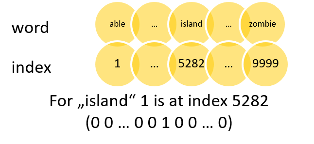
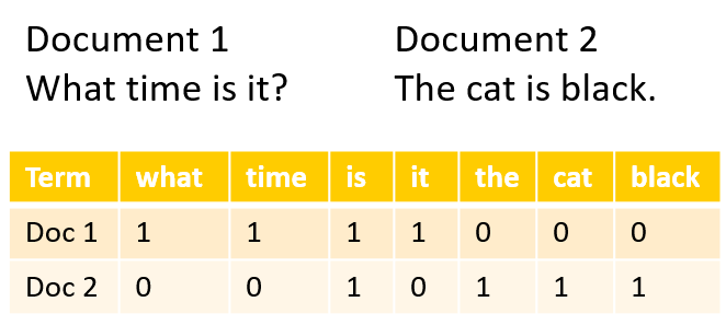
FIGURE 2.1: One-Hot Encoding on the left and Bag-of-Words on the right. Source: Own figure.

The solution to this problem is word embedding. Word embeddings use dense vector representations for words. That means they map each word to a continuous vector with n dimensions. The distance in the vector space denotes semantic (dis)similarity. These word embeddings are usually learned by neural networks, either within the final model in an additional layer or in its own model. Once learned they can be reused across different tasks. Practically all NLP projects these days build upon word embeddings, since they have a lot of advantages compared to the aforementioned representations. The basic idea behind learning word embeddings is the so called “distributional hypothesis” (see Harris (1954)). It states that words that occur in the same contexts tend to have similar meanings. The two best known approaches for calculating word embeddings are Word2vec from Tomas Mikolov, Sutskever, et al. (2013) and GloVE from Pennington et al. (2014). The Word2vec models (Continous Bag-Of-Words (CBOW) and Skip-gram) try to predict a target word given his context or context words given a target word using a simple feed-forward neural network. In contrast to these models GloVe not only uses the local context windows, but also incorporates global word co-occurrence counts. As mentioned, a lot of approaches use neural networks to learn word embeddings. A simple feed-forward network with fully connected layers for learning such embeddings while predicting the next word for a given context is shown in figure 2.2. In this example the word embeddings are first learnt in a projection layer and are then used in two hidden layers to model the probability distribution over all words in the vocabulary. With this distribution one can predict the target word. This simple structure can be good enough for some tasks but it also has a lot of limitations. Therefore, recurrent and convolutional networks are used to overcome the limitations of a simple neural network.

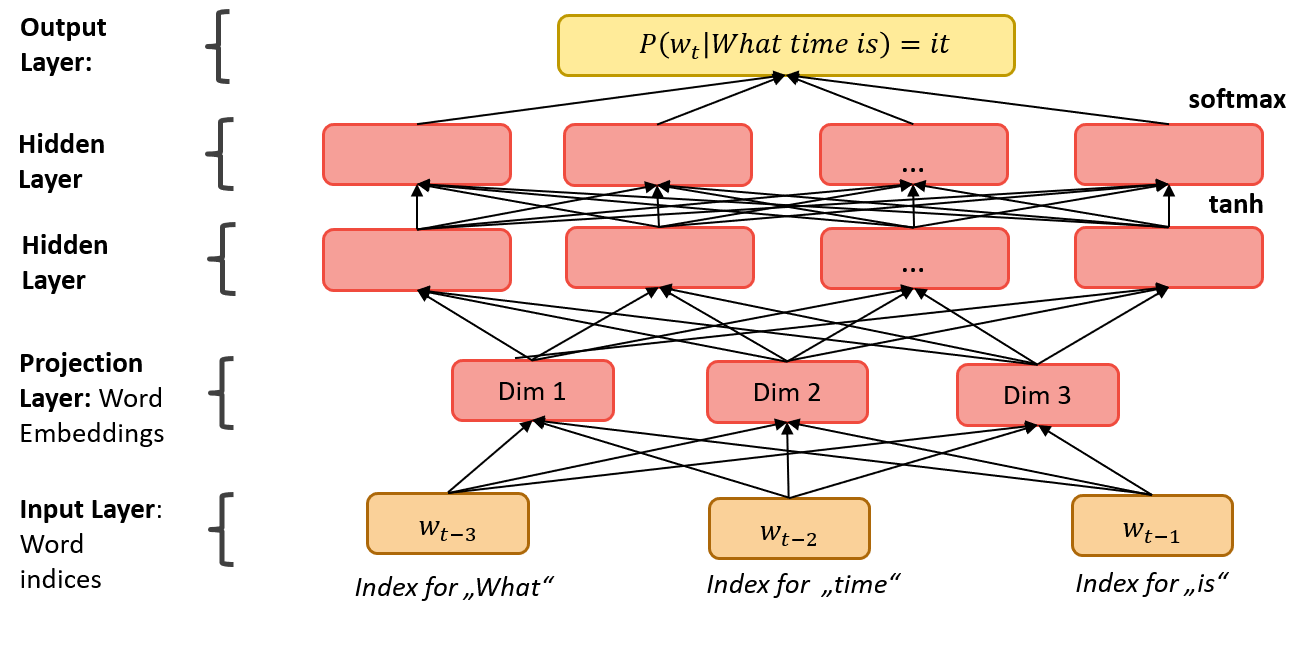
FIGURE 2.2: Feed-forward Neural Network. Source: Own figure based on Bengio et al. 2013.

2.2 Recurrent Neural Networks

The main drawback of feedforward neural networks is that they assume a fixed length of input and output vectors which is known in advance. But for many natural language problems such as machine translation and speech recognition it is impossible to define optimal fixed dimensions a-priori. Other models that map a sequence of words to another sequence of words are needed (Sutskever, Vinyals, and Le 2014). Recurrent neural networks or RNNs are a special family of neural networks which were explicitely developed for modeling sequential data like text. RNNs process a sequence of words or letters \(x^{(1)}, ..., x^{(t)}\) by going through its elements one by one and capturing information based on the previous elements. This information is stored in hidden states \(h^{(t)}\) as the network memory. Core idea is rather simple: we start with a zero vector as a hidden state (because there is no memory yet), process the current state at time \(t\) as well as the output from the previous hidden state, and give the result as an input to the next iteration (Goodfellow, Bengio, and Courville 2016).

Basically, a simple RNN is a for-loop that reuses the values which are calculated in the previous iteration (Chollet 2018). An unfolded computational graph (figure 2.3) can display the structure of a classical RNN. The gray square on the left represents a delay of one time step and the arrows on the right express the flow of information in time (Goodfellow, Bengio, and Courville 2016).

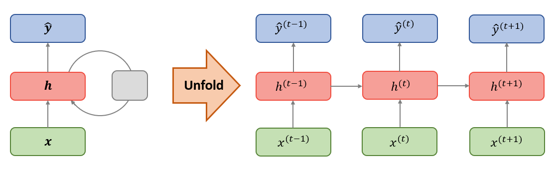
FIGURE 2.3: Right: Circuit diagram (left) and unfolded computational graph (right) of a simple RNN. Source: Own figure.

One particular reason why recurrent networks have become such a powerful technique in processing sequential data is parameter sharing. Weight matrices remain the same through the loop and they are used repeatedly, which makes RNNs extremely convenient to work with sequential data because the model size does not grow for longer inputs. Parameter sharing allows application of models to inputs of different length and enables generalization across different positions in real time (Goodfellow, Bengio, and Courville 2016).

As each part of the output is a function of the previous parts of the output, backpropagation for the RNNs requires recursive computations of the gradient. The so-called backpropagation through time or BPTT is rather simple in theory and allows for the RNNs to access information from many previous steps (Boden 2002). In practice though, RNNs in their simple form are subject to two big problems: exploding and vanishing gradients. As the gradients are computed recursively, they may become either very small or very large, which leads to a complete loss of information about long-term dependencies. To avoid these problems, gated RNNs were developed and accumulation of information about specific features over a long duration became possible. The two most popular types of gated RNNs, which are widely used in modern NLP, are Long Short-Term Memory models (LSTMs, presented by Hochreiter and Schmidhuber (1997)) and Gated Recurrent Units (GRUs, presented by Cho et al. (2014)).

Over last couple of years, various extentions of RNNs were developed which resulted in their wide application in different fields of NLP. Encoder-Decoder architectures aim to map input sequences to output sequences of different length and therefore are often applied in machine translation and question answering (Sutskever, Vinyals, and Le 2014). Bidirectional RNNs feed sequences in their original as well as reverse order because the prediction may depend on the future context, too (Schuster and Paliwal 1997). Besides classical tasks as document classification and sentiment analysis, more complicated challenges such as machine translation, part-of-speech tagging or speech recognition can be solved nowadays with the help of advanced versions of RNNs.

2.3 Convolutional Neural Networks

Throughout machine learning or deep learning algorithms, no one algorithm is only applicable to a certain field. Most algorithms that have achieved significant results in a certain field can still achieve very good results in other fields after slight modification. We know that convolutional neural networks (CNN) are widely used in computer vision. For instance, a remarkable CNN model called AlexNet achieved a top-5 error of 15.3% in the ImageNet 2012 Challenge on 30 September 2012 (see Krizhevsky, Sutskever, and Hinton (2012)). Subsequently, a majority of models submitted by ImageNet teams from around 2014 are based on CNN. After the convolutional neural network achieved great results in the field of images, some researchers began to explore convolutional neural networks in the field of natural language processing (NLP). Early research was restricted to sentence classification tasks, CNN-based models have achieved very significant effects as well, which also shows that CNN is applicable to some problems in the field of NLP. Similarly, as mentioned before, one of the most common deep learning models in NLP is the recurrent neural network (RNN), which is a kind of sequence learning model and this model is also widely applied in the field of speech processing. In fact, some researchers have tried to implement RNN models in the field of image processing, such as (Visin et al. (2015)). It can be seen that the application of CNN or RNN is not restricted to a specific field.

As the Word2vec algorithm from Tomas Mikolov, Sutskever, et al. (2013) and the GloVe algorithm from Pennington et al. (2014) for calculating word embeddings became more and more popular, applying this technique as a model input has become one of the most common text processing methods. Simultaneously, significant effectiveness of CNN in the field of computer vision has been proven. As a result, utilizing CNN to word embedding matrices and automatically extract features to handle NLP tasks appeared inevitable.

The following figure 2.4 illustrates a basic structure of CNN, which is composed of multiple layers. Many of these layers are described and developed with some technical detail in later chapters of this paper.

FIGURE 2.4: Basic structure of CNN. Source: Own figure.

It is obvious that neural networks consist of a group of multiple neurons (or perceptron) at each layer, which uses to simulate the structure and behavior of biological nervous systems, and each neuron can be considered as logistic regression.

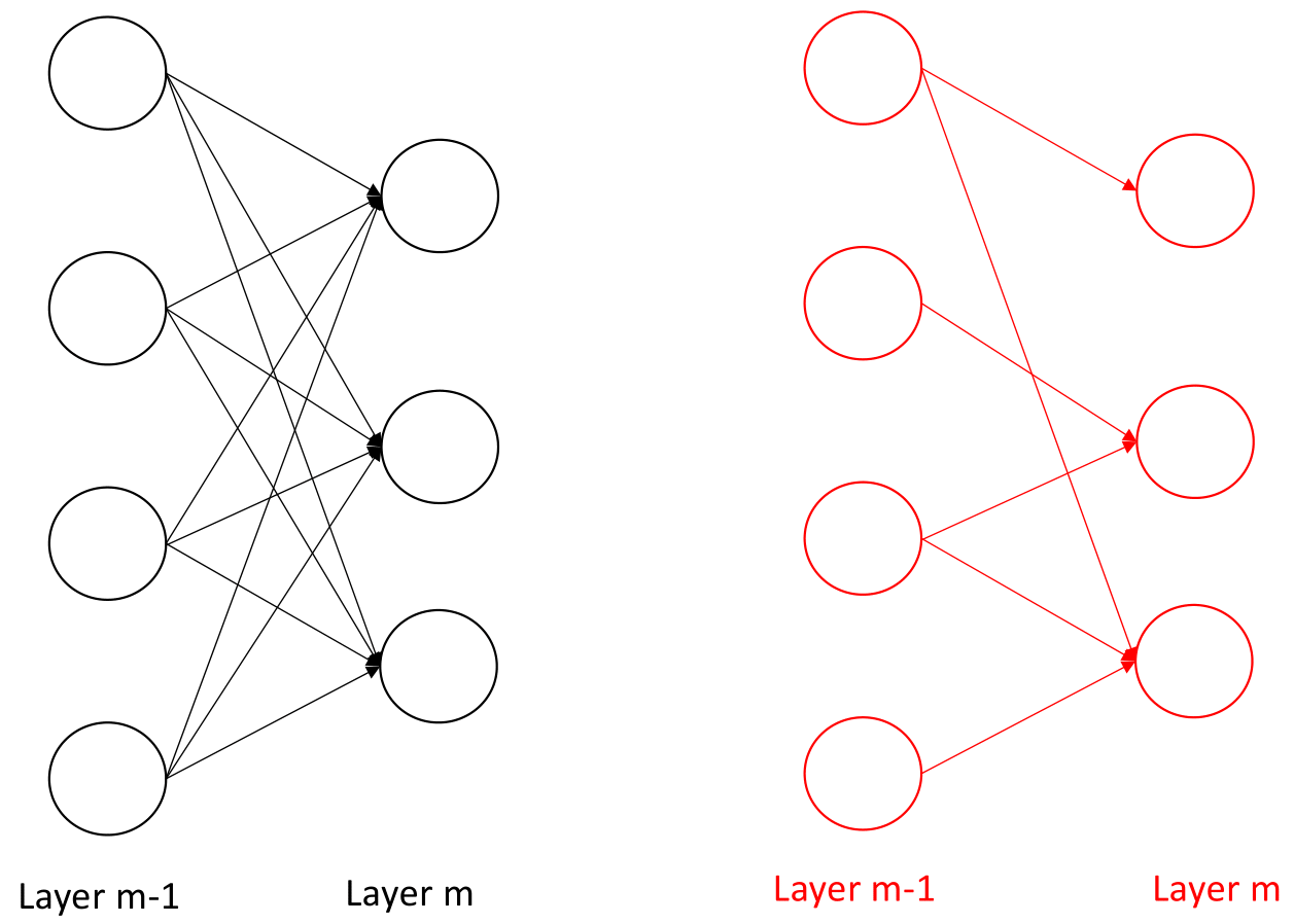
FIGURE 2.5: Comparison between the fully-connected and partial connected architecture. Source: Own figure.

The structure of CNN is different compared with traditional neural networks as illustrated in figure 2.5. In traditional neural networks structure, the connections between neurons are fully connected. To be more specific, all of the neurons in the layer \(m-1\) are connected to each neuron in the layer \(m\), but CNN sets up spatially-local correlation by performing a local connectivity pattern between neurons of neighboring layers, which means that the neurons in the layer \(m-1\) are partially connected to the neurons in the layer \(m\). In addition to this, the left picture presents a schematic diagram of fully-connected architecture. It can be seen from the figure that there are many edges between neurons in the previous layer to the next layer, and each edge has parameters. The right side is a local connection, which shows that there are relatively few edges compared with fully-connected architecture and the number of visible parameters has significantly decreased.

A detailed description of CNN will be presented in the later chapters and the basic architecture of if will be further explored. Subsection 5.1 gives an overview of CNN model depends upon (Kim (2014)). At its foundation, it is also necessary to explain various connected layers, including the convolutional layer, pooling layer, and so on. In 5.2 and later subsections, some practical applications of CNN in the field of NLP will be further explored, and these applications are based on different CNN architecture at diverse level, for example, exploring the model performance at character-level on text classification research (see Zhang, Zhao, and LeCun (2015)) and based on multiple data sets to detect the Very Deep Convolutional Networks (VD-CNN) for text classification (see Schwenk et al. (2017)).

References

Bengio, Yoshua, Réjean Ducharme, Pascal Vincent, and Christian Jauvin. 2003. “A Neural Probabilistic Language Model.” Journal of Machine Learning Research, no. 3: 1137–55.

Boden, Mikael. 2002. “A Guide to Recurrent Neural Networks and Backpropagation.” The Dallas Project.

Cho, Kyunghyun, Bart Van Merriënboer, Caglar Gulcehre, Dzmitry Bahdanau, Fethi Bougares, Holger Schwenk, and Yoshua Bengio. 2014. “Learning Phrase Representations Using Rnn Encoder-Decoder for Statistical Machine Translation.” arXiv Preprint arXiv:1406.1078.

Chollet, Francois. 2018. Deep Learning Mit Python Und Keras: Das Praxis-Handbuch Vom Entwickler Der Keras-Bibliothek. MITP-Verlags GmbH & Co. KG.

Goodfellow, Ian, Yoshua Bengio, and Aaron Courville. 2016. Deep Learning. MIT press.

Harris, Zellig S. 1954. “Distributional Structure.” WORD 10 (2-3): 146–62.

Hochreiter, Sepp, and Jürgen Schmidhuber. 1997. “Long Short-Term Memory.” Neural Computation 9 (8). MIT Press: 1735–80.

Kim, Yoon. 2014. Convolutional Neural Networks for Sentence Classification. https://www.aclweb.org/anthology/D14-1181.pdf.

Krizhevsky, Alex, Ilya Sutskever, and Geoffrey E. Hinton. 2012. ImageNet Classification with Deep Convolutional Neural Networks. http://www.cs.toronto.edu/~hinton/absps/imagenet.pdf.

Mikolov, Tomas, Ilya Sutskever, Kai Chen, Greg Corrado, and Jeffrey Dean. 2013. “Distributed Representations of Words and Phrases and Their Compositionality.” Advances in Neural Information Processing Systems, 3111–9.

Pennington, Jeffrey, Richard Socher, Manning, and Christopher D. 2014. “GloVe: Global Vectors for Word Representation.” Proceedings of the 2014 Conference on Empirical Methods in Natural Language Processing (EMNLP), 1532–43.

Schuster, Mike, and Kuldip K Paliwal. 1997. “Bidirectional Recurrent Neural Networks.” IEEE Transactions on Signal Processing 45 (11). Ieee: 2673–81.

Schwenk, Holger, Loïc Barrault, Alexis Conneau, and Yann LeCun. 2017. Very Deep Convolutional Networks for Text Classification. https://www.aclweb.org/anthology/E17-1104.pdf.

Sutskever, Ilya, Oriol Vinyals, and Quoc V Le. 2014. “Sequence to Sequence Learning with Neural Networks.” In Advances in Neural Information Processing Systems, 3104–12.

Visin, Francesco, Kyle Kastner, Kyunghyun Cho, Matteo Matteucci, Aaron C. Courville, and Yoshua Bengio. 2015. ReNet: A Recurrent Neural Network Based Alternative to Convolutional Networks. ArXiv. Vol. abs/1505.00393.

Zhang, Xiang, Junbo Jake Zhao, and Yann LeCun. 2015. Character-Level Convolutional Networks for Text Classification. https://papers.nips.cc/paper/5782-character-level-convolutional-networks-for-text-classification.pdf.