Chapter 3 Foundations/Applications of Modern NLP

Authors: Viktoria Szabo

Supervisor: Christian Heumann

Word embeddings can be seen as the beginning of modern natural language processing. They are widely used in every kind of NLP task. One of the advantages is that one can download and use pretrained word embeddings. With this, it is possible to save a lot of time for training the final model. But if the task is not a standard one it is usually better to train own embeddings to get a better model performance for the specific task. In the following the evolution from sparse representations of words to dense word embeddings will be outlined in the first part. After that the calculation methods for word embeddings within a neural network language model and with word2vec and GloVe will be described. The third part shows how to improve the model performance regardless of the chosen model class based on hyperparameter tuning and system design choices and explains some model expansion to tackle problems of the aforementioned methods. The evaluation of word embeddings on different tasks and datasets is another topic which will be covered in the fourth part of this chapter. Finally some resources to download pretrained word embeddings will be presented.

3.1 The Evolution of Word Embeddings

Since computers work with numeric representations, converting the text and sentences to be analyzed into numbers is unavoidable. One-Hot Encoding and Bag-of-Words (BOW) are two simple approaches to how this could be accomplished. These methods are usually used as input for calculating more elaborate word representations called word embeddings.
The One-Hot Encoding labels each word in the vocabulary with an index. Let \(n\) be size of the vocabulary, then each word is represented by a vector with dimension \(n\). Every vector entry is zero except for the one corresponding to its index, which is set to \(1\). A sentence is represented as a matrix of shape (\(n\times n\)) where \(n\) is the number of unique words in the sentence or a document. In figure 3.1 an example for a one-hot encoded word is shown on the left side.
A more elaborate approach compared to the first one is called Bag-of-Words (BOW) and belongs to the count-based approaches. This approach counts the occurrences and co-occurrences of all distinct words in a document or a text chunk. Each text chunk is then represented by a row in a matrix, where the columns are the words. That means that, compared to the One-Hot Encoding, this approach already incorporates some context information in sentences and text chunks. An example for this kind of representation can be seen on the right side in figure 3.1.

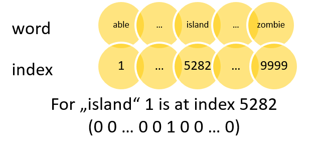
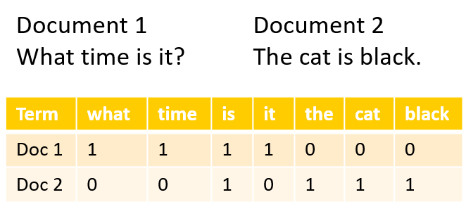
FIGURE 3.1: One-Hot Encoding on the left and Bag-of-Words on the right. Source: Own figure.

These approaches definitely have some positive points about them. They are very simple to construct, robust to changes, and it was observed that simple models trained on large amounts of data outperform complex systems trained on less data. Bag-of-Words is especially useful if the number of distinct words is small and the sequence of the words doesn’t play a key role, like in sentiment analysis. Without calculating word embeddings on top of them, these approaches should only be used if there is a small number of distinct words in the document, the words are not meaningfully correlated and there is a lot of data to learn from.
Nevertheless, the problems that arise from these approaches usually outweigh the positive points. The most obvious one is that these approaches lead to very sparse input vectors, that means large vectors with relatively few non-zero values. Many machine learning models won’t work well with high dimensional and sparse features (Goldberg (2016)). Neural networks in particular struggle with this type of data. And with growing vocabulary the feature size vectors also increases by the same length. So, the dimensionality of these approaches is the same as the number of different words in your text. That means estimating more parameters and therefore using exponentially more data is required to build a reasonably generalizable model. This is known as the curse of dimensionality. But these problems can be solved with dimensionality reduction methods such as Principal Component Analysis or feature selection models where less informative context words, such as the and a are dropped.
The major drawback of these methods is that there is no notion of similarity between words. That means words like cat and tiger are represented as similar as cat and car. If the words cat and tiger would be represented as similar words one could use the information won from the more frequent word “cat” for sentences in which the less frequent word tiger appears. If the word embedding for tiger is similar to that of cat the network model can take a similar path instead of having to learn how to handle it completely anew.

To overcome these problems word embeddings were introduced. Word embeddings use continuous vectors to represent each word in a vocabulary. These vectors have \(n\) dimensions, usually between 100 and 500, which represent different aspects of the word. With this approach, semantic similarity can be maintained in the representation and generalization may be achieved. Through these vectors, the words are mapped to a continuous vector space, called a semantic space, where semantically similar words occur close to each other, while more dissimilar words are far from each other. Figure 3.2 shows a simple example to convey the idea behind this approach. In this fictional example the words are represented by a two-dimensional vector, which represents the cuteness and scariness of the creatures.

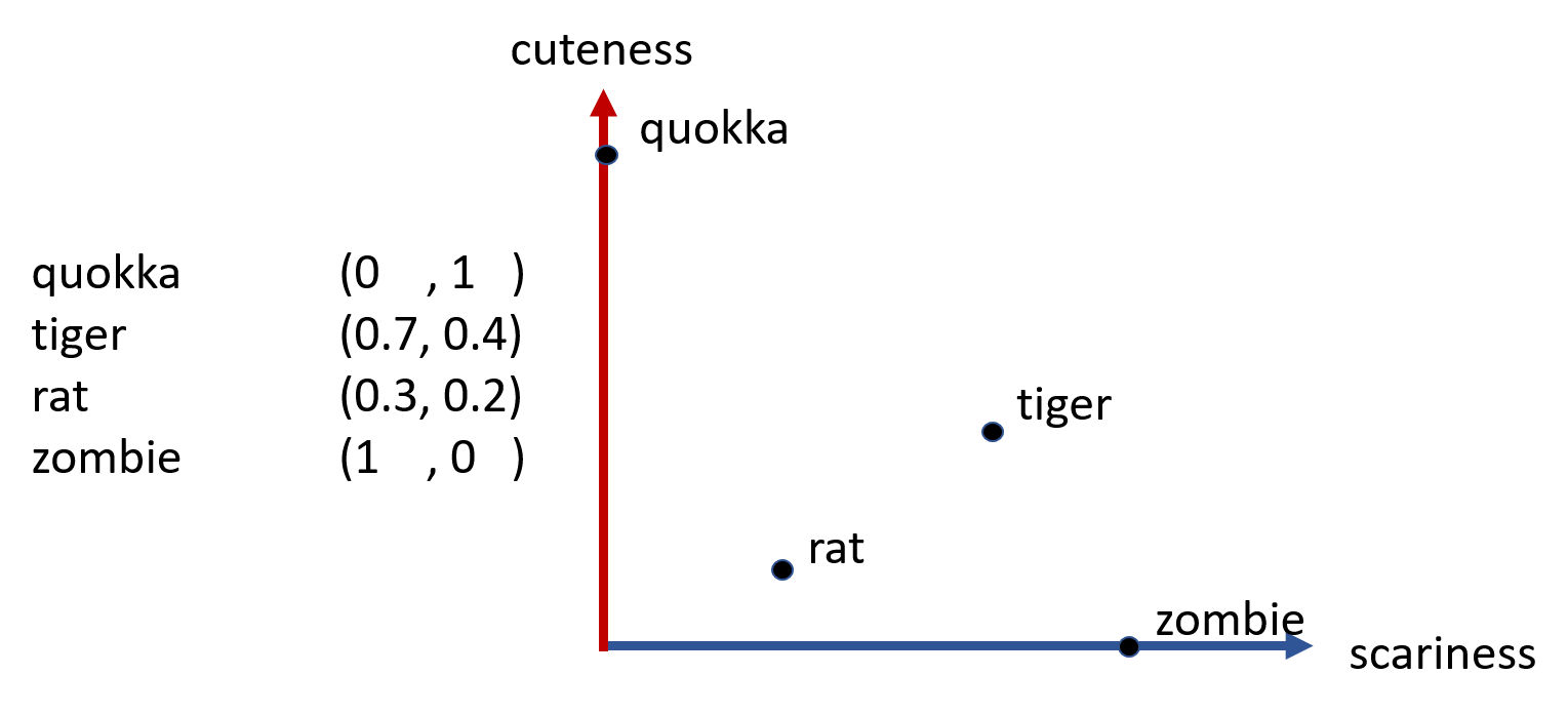
FIGURE 3.2: Example for word embeddings with two dimensions. Source: Own figure

If the goal is to represent higher dimensional word vectors one could use dimension reduction methods such as principal component analysis (PCA) to break down the number of dimensions into two or three and then plot the words. There is an example of this for selected country names and their capitals in figure 3.3.The country names all have negative values on the x-axis and the capitals all have positive values on the x-axis. Furthermore, the countries have y-axis values similar to their corresponding capitals.

FIGURE 3.3: Two-dimensional PCA projection of 1000-dimensional word vectors of countries and their capital cities. Source: Tomas Mikolov, Sutskever, et al. (2013)

With such word vectors even algebraic computations become possible as shown in Tomáš Mikolov, Yih, and Zweig (2013). For example, \(vector(King)-vector(Man) + vector(Woman)\) results in a vector that is closest to the vector representation of the word Queen. Another possibility to use word embeddings vectors is translation between languages. Tomas Mikolov, Le, and Sutskever (2013) showed that they can find word translations by comparing vectors generated from different languages. By searching for a translation one can use the word vector from the source language and search for the closest vector in the target language vector space, this word can then be used as a translation. The reason this works is that if a word vector from one language is similar to the word vector of the other language, this word is used in a similar context. This method can be used to infer missing dictionary entries. An example for this method depicted in figure 3.4. In figure 3.4 the vectors for numbers and animals are depicted on the left side and the same words are depicted on the right side. It can be seen that the vectors for the correct translation align in similar geometric spaces. Again, two-dimensional representation was achieved by using dimension reduction methods.

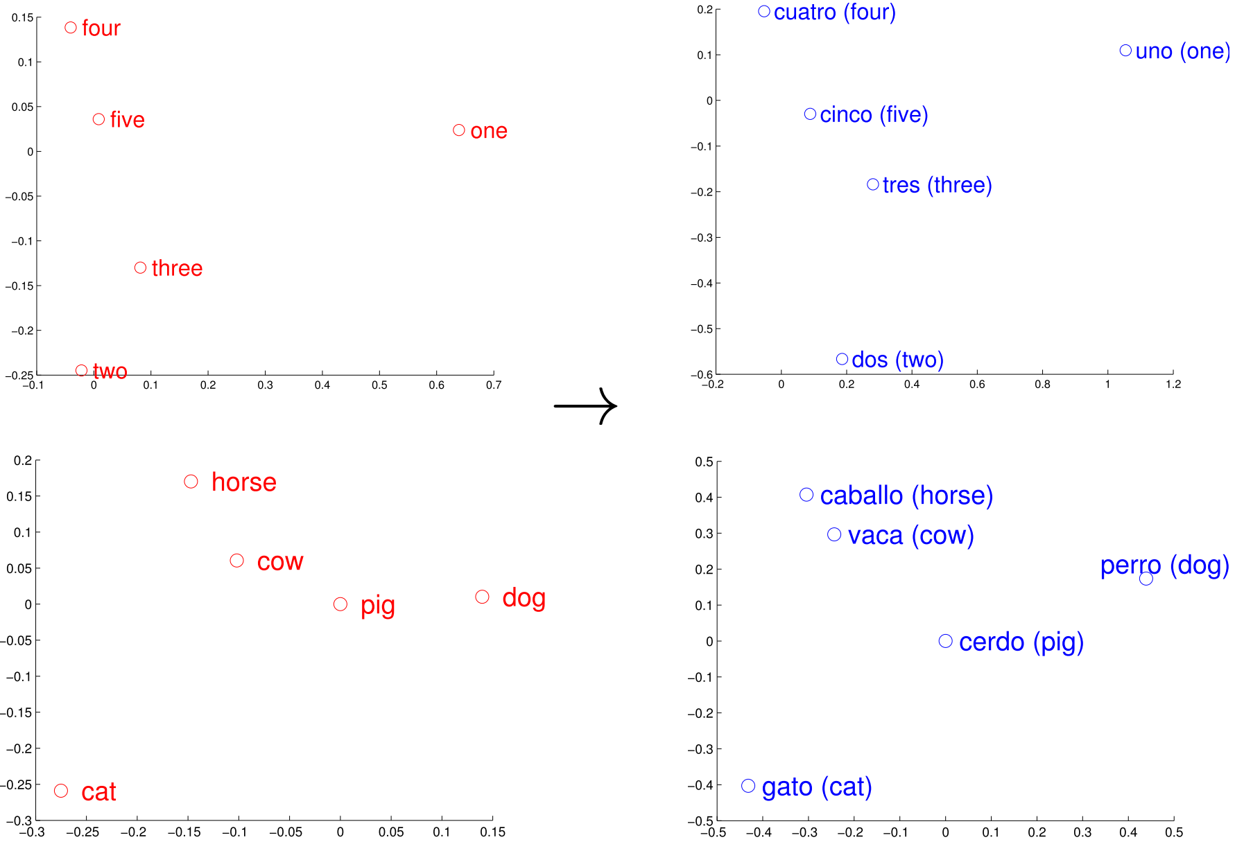
FIGURE 3.4: Distributed word vector representations of numbers and animals in English (left) and Spanish (right). Source: Tomas Mikolov, Le, and Sutskever (2013)

3.2 Methods to Obtain Word Embeddings

The basic idea behind learning word embeddings is the so called distributional hypothesis (Harris (1954)). It states that words that occur in the same contexts tend to have similar meanings. For instance, the words car and truck tend to have similar semantics as they appear in similar contexts, e.g., with words such as road, traffic, transportation, engine, and wheel. Hence machine learning and deep learning algorithms can find representations by themselves by evaluating the context in which a word occurs. Words that are used in similar contexts will be given similar representations. This is usually done as an unsupervised or self-supervised procedure, which is a big advantage. That means word embeddings can be thought of as unsupervised feature extractors for words. However, the methods to find such similarities in the context of words vary. Finding word representations started out with more traditional count-based techniques, which collected word statistics like occurrence and co-occurrence frequencies as seen above with BOW. But these representations often require some sort of dimensionality reduction. Later, when neural networks were introduced into NLP, the so-called predictive techniques, mainly popularized after 2013 with the introduction of word2vec, supplanted the traditional count-based word representations.These models learn what is called dense representations of words, since they directly learn low-dimensional word representations, without needing the additional dimensionality reduction step. In the following an introduction to the best-known predictive approaches to model word embeddings will be given. First, neural network language models, where word embeddings are learnt as a part of the final language model will be discussed. The description of the two popular algorithms word2vec and GloVe, which learn word embeddings in a pre-step before the actual statistical language model, follow afterwards.

3.2.1 Feedforward Neural Network Language Model (NNLM)

Bengio et al. (2003) were the first to propose learning word embeddings within a statistical neural network language model (NNLM). The goal of the NNLM model of Bengio et al. (2003) is to predict the next word based on a sequence of preceding words. Using a simple feedforward neural network, the model first learns the word embeddings and in a second step the probability function for word sequences. This way, one obtains not only the model itself, but also the learned word representations, which can be used as input for other, potentially unrelated, tasks.
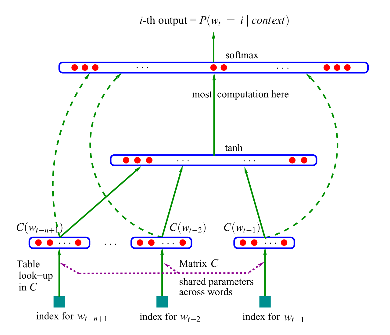
The proposed neural network architecture has an input layer with one-hot encoded word inputs, a linear projection layer for the word embeddings, and a hidden layer with a hyperbolic tangent function, where most of the computation is done, followed by a softmax classifier output layer. The output of the model is a vector of the probability distribution over all words given a specific context. That means a vector with probability scores for each word of the vocabulary. The i-th element of the output vector is the probability estimation \(P(w_t = i|context)\). The softmax classifier is used to guarantee positive probabilities summing to one. It computes the following function: \[\widehat{P}(w_t|w_{t-1},...,w_{t-n+1}) = \frac{ e^{Y_{w_t}} }{ \sum_{i} {e^{y_i}} }\] The \(y_i\) are the unnormalized log-probabilities for each output word \(i\), which were computed in the previous layer. The model architecture proposed in Bengio et al. (2003) is depicted in figure 3.5.
When training a neural network, one has to define a loss function \(L(\widehat{y}, y)\) stating the loss of predicting \(\widehat{y}\) when the true output is \(y\). In the NNLM literature, a cross-entropy loss is very common (see Goldberg (2016)). The \(\widehat{y}\) is the network output vector, which was transformed by the softmax classifier and represents the conditional distribution. The \(y\) is usually either a one-hot vector for the correct output word or a vector representing the true multinomial probability distribution over the vocabulary given the specific context. Then the parameter \(\phi\) of the neural network (for example the weights for the embedding vectors) is iteratively changed in order to minimize the loss \(L\) over the training examples.
This is usually done with the stochastic gradient descent (SGD) optimizer where the gradient is obtained via backpropagation. The gradient descent optimizer tries to find the direction of the strongest descent via partial derivatives and updates the parameter \(\phi\) accordingly. The learning rate \(\varepsilon\) defines the size of the step in this direction (see Goldberg (2016)).
In Bengio et al. (2003) a gradient ascent optimizer is used, which performs the following iterative update after presenting the t-th word of the training corpus: \[\theta \leftarrow \theta + \varepsilon\frac{\partial log\widehat{P}(w_t|w_{t-1},...,w_{t-n+1})}{\partial \theta }\] The method by which parameter adjustments are made during training so they can be optimized is called backpropagation. Backpropagation essentially consists of six steps:

1. Initialization of the parameter of the network
2. Calculation of \(y(x_i)\) for the inputs \(x_i\)
3. Determining the cost of the inputs \(x_i\)
4. Calculation of the partial derivatives of the loss for each parameter
5. Update the parameter in the network using the partial derivatives calculated in step 4
6. Return to step 2 and continue the procedure until the partial derivatives of the loss approach zero

FIGURE 3.5: Architecture for NNLM proposed by Bengio et al. (2003) . Source: Bengio et al. (2003)

3.2.2 Word2Vec

In 2013 Tomas Mikolov, Chen, et al. (2013) proposed the two word2vec algorithms which led to a wave in NLP that popularized word embeddings. In contrast to the NNLM model above, the word2vec algorithms are not used for a statistical language modeling goal, but rather to learn the word embeddings themselves. The two word2vec algorithms named Continuous Bag-of-Words (CBOW) and Continuous Skip-Gram use shallow neural networks with an input layer, a projection layer, and an output layer. This means compared to the previously explained feedforward NNLM, the non-linear hidden layer is removed.
The general idea behind CBOW is to predict the focus word based on a window of context words. The order of context words does not influence the prediction, thus the name Bag-of-Words. In contrast, Skip-Gram tries to predict the context words given a source word. This is done while adjusting the initial weights during training so that a loss function is reduced.
In the CBOW architecture the \(N\) input (context) words are each one-hot encoded vectors of size \(V\), where \(V\) is the size of the vocabulary. Compared to the NNLM model CBOW uses both previous and following words as context instead of only the previous words. The projection layer is a standard fully connected (dense) layer which has the dimensionality \(1 \times D\), where \(D\) is the size of the dimensions for the word embeddings. The projection layer is shared for all words. That means all words get projected into the same position in a linear manner, where the vectors are averaged. The output layer outputs probabilities for the target words from the vocabulary and has a dimensionality of \(V\). That means the output is a probability distribution over all words of the vocabulary as in the NNLM model, where the prediction is the word with the highest probability. But instead of using a standard softmax classifier as in the NNLM model the authors propose to use a log-linear hierarchical softmax classifier for the calculation of the probabilities. The model architecture is shown in figure 3.6. The continuous Skip-gram architecture also uses a log-linear hierarchical softmax classifier with a continuous projection layer, but the input is only one source word, and the output layer consists of as many probability vectors over all words as the chosen number of context words. Also, since the more distant words are usually less related to the source word, the skip-gram model weighs nearby context words more heavily than more distant context words by sampling less from those words in the training examples. The model architecture for skip-gram can be found on the right side of figure 3.6.

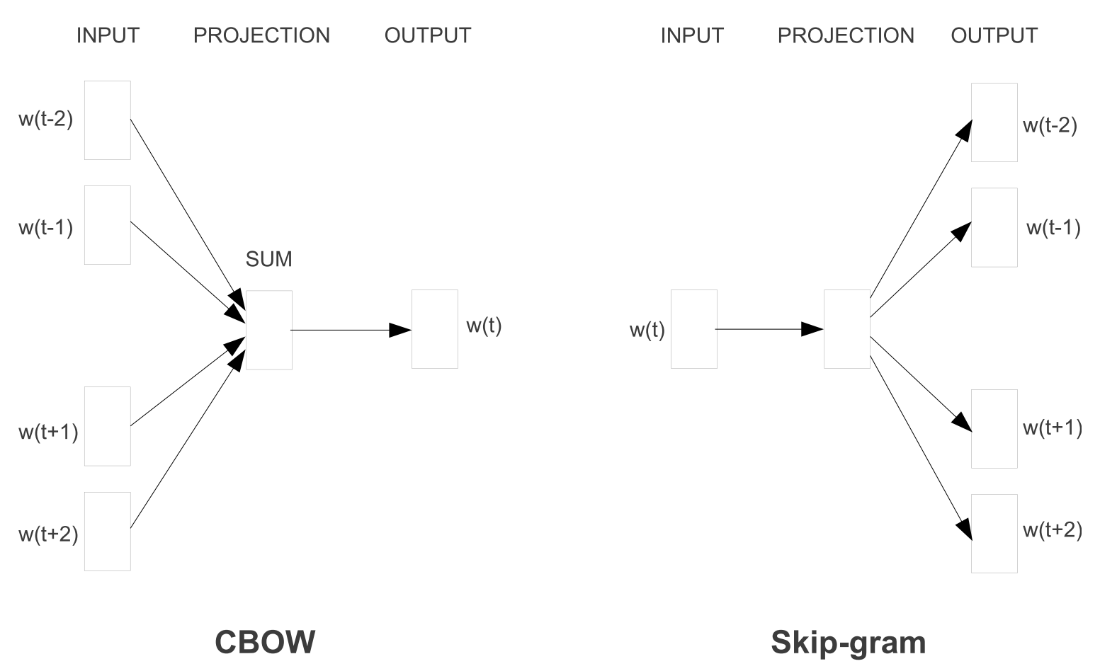
FIGURE 3.6: Learning word embeddings with the model architecture of CBOW and Skip-Gram. Source: Tomas Mikolov, Chen, et al. (2013)

As said before the word2vec models use hierarchical softmax, where the vocabulary is represented as a Huffman binary tree, instead of the standard softmax classifier explained in the section before. With hierarchical softmax the size of the output vector can be reduced from the vocabulary size \(V\) to the logarithm to base 2 of \(V\), which is a dramatic change in computational complexity and number of operations needed for the algorithm. Further explanations for this method can be found in Morin and Bengio (2005). For both models Tomas Mikolov, Chen, et al. (2013) use gradient descent optimization and backpropagation as described in the previous chapter.
Tomas Mikolov, Chen, et al. (2013) show that their word2vec algorithms outperform a lot of other standard NNLM models. CBOW is faster while skip-gram does a better job for infrequent words. Skip-gram works well with small amounts of training data and has good representations for words that are considered rare, whereas CBOW trains several times faster and has slightly better accuracy for frequent words.

3.2.3 GloVe

GloVe stands for Global Vector word representation, which emphasizes the global character of this model. Unlike the previously described algorithms like word2vec, GloVe not only relies on local context information but also incorporates global co-occurrence statistics. Instead of extracting the embeddings from a neural network that is designed to perform a task like predicting neighboring words (CBOW) or predicting the focus word (Skip-Gram), the embeddings are optimized directly, so that the dot product of two word vectors is equal to the log of the number of times the two words will occur near each other. The model builds on the possibility to derive semantic relationships between words from the co-occurrence matrix and that the ratio of co-occurrence probabilities of two words with a third word is more indicative of semantic association than a direct co-occurrence probability (see Pennington et al. (2014)).
Let \(P_{ij} = P(j|i) = X_{ij}/X_i\) be the probability that word \(j\) appears in the context of word \(i\). Figure 3.7 shows an example with the words ice and steam. The relationship of these words can be examined by studying the ratio of their co-occurrence probabilities with other words \(k\).
For words like solid which are related to ice but not steam the ratio is large (>1), while for words like gas, which is related to steam but not to ice, the ratio is small (<1). For words like water or fashion, which are either related to both of the words or to none the ratios are close to 1. It is evident that the comparison of co-occurrence probabilities with a third word (\(P_{ik}/P_{jk}\)) is more indicative of the semantic meanings of words \(i\) and \(j\) and is better at identifying words (solid and gas) that distinguish \(i\) and \(j\) and words that do not (water and fashion) than the raw probabilities.

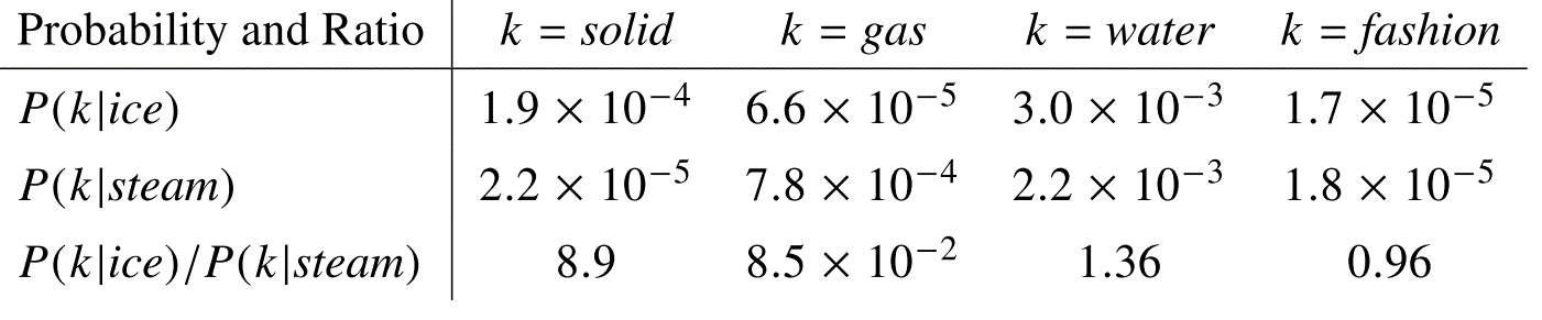
FIGURE 3.7: Co-occurrence probabilities for target words ice and steam with selected context words. Source: Pennington et al. (2014)

Pennington et al. (2014) tried to incorporate the ratio \(P_{ik}/P_{jk}\) into computing word embeddings. They propose an optimization problem which aims at fulfilling the following objective: \[w_i^Tw_k + b_i + b_k = log(X_{ik})\] Where \(b_i\) and \(b_k\) are bias terms for word \(w_i\) and probe word \(w_k\) and \(X_{ik}\) is the number of times \(w_i\) co-occurs with \(w_k\). Fulfilling this objective minimizes the difference between the dot product of \(w_i\) and \(w_k\) and the logarithm of their number of co-occurrences. In other words, the optimization results in the construction of vectors \(w_i\) and \(w_k\) whose dot product gives a good estimate of their transformed co-occurrence counts. To solve this optimization problem, they reformulate the equation as a least squares problem and introduce a weighting function, since rare co-occurrences add both noise to the model and less information than more frequent co-occurrences.

3.3 Hyperparameter Tuning and System Design Choices

Once adapted across methods, hyperparameter tuning significantly improves performance in every task. Levy, Goldberg, and Dagan (2015) showed that in a lot of cases, changing the setting of a single hyperparameter could yield a greater increase in performance than switching to a better algorithm or training on a larger corpus. They conducted a series of experiments where they assessed the contributions of diverse hyperparameters. They also show that when all methods are allowed to tune a similar set of hyperparameters, their performance is largely comparable. However they also found that choosing the wrong hyperparameter settings can actually degrade performance of a model. That is why tuning the hyperparameter fitting the specific context is very important. Depending on the model one chooses there are a lot of hyperparameters available for tuning. These are parameters like the number of epochs, batch-size, learning rate, embedding size, window size, corpus size et cetera. In the following the focus will lie on hyperparameters which are frequently discussed. Furthermore, some system design and setup choices will be described which will tackle some of the problems posed by the algorithms mentioned above.

Word embedding size
The question of how many embedding dimensions should be used is mostly answered empirically. It depends on the task, computing capacity and vocabulary. The trade-off is between accuracy and computational concerns. More dimensions could potentially increase the accuracy of the representations; since the vectors can capture more aspects of the word. But more dimensions also mean higher computing time and effort. In practice word embedding vectors with dimensions around 50 to 300 are usually used as a rule of thumb (see Goldberg (2016)).
In contrast, Patel and Bhattacharyya (2017) found that the dimension size should be chosen based on some text corpus statistics. One can calculate a lower bound from the number of pairwise equidistant words of the corpus vocabulary. Choosing a dimension size below this bound results in a loss of quality of learned word embeddings. This result was tested empirically for the skip-gram algorithm (see Patel and Bhattacharyya (2017)).
Pennington et al. (2014) compare performance of the GloVe model for embedding sizes from 1 to 600 for different evaluation tasks (semantic, syntactic and overall). They found that after around 200 dimensions the performance increase begins to stagnate.

Context Window
In traditional approaches the context window around the focus word is constant-sized and unweighted. For example, if the symmetrical context size is 5 then the 5 words before the focus word and 5 words after the focus words are the context window. It is also possible to use an asymmetric context window, which for example only uses words that appear before the focus word. A window size of 5 is commonly used to capture broad topic/domain information like what other words are used in related discussions (i.e. dog, bark and leash will be grouped together, as well as walked, run and walking), whereas smaller windows contain more specific information about the focus word and produce more functional and syntactic similarities (i.e. Poodle, Pitbull, Rottweiler, or walking, running, approaching) (see Goldberg and Levy (2014), Goldberg (2016)).
Since words which appear closer to the focus word are usually more indicative of its meaning it is possible to give the context words weights according to their distance from the focus word. Both word2vec and GloVe use such weighting schemes. GloVe’s implementation weights contexts using the harmonic function, e.g. a context word three tokens away will have 1/3 as a weight. Word2vec’s uses weightings of the distance from the focus word divided by the window size. For example, a size-5 window will weigh its contexts by \(\frac {5}{5}\), \(\frac {4}{5}\), \(\frac {3}{5}\), \(\frac {2}{5}\), \(\frac {1}{5}\) (Levy et al. 2015).
A performance comparison for GloVe using different window sizes for different evaluation tasks (semantic, syntactic and overall) can be found in Pennington et al. (2014). Which shows that, depending on the task, larger performance gains can be expected from a larger window size. But for all three tasks the performance gains decrease after a window size of 4.

Document Context
Instead of using a few words as the context window one could consider all the other words that appear with the focus word in the same sentence, paragraph, or document. One can either consider this as using very large window sizes or, as in the doc2vec algorithm from Le and Mikolov (2014), add another embedding vector for a whole paragraph to the other context word vectors. These approaches will result in word vectors that capture topical similarity (words from the same topic, i.e. words that one would expect to appear in the same document, are likely to receive similar vectors). (Goldberg (2016); Le and Mikolov (2014))

Subsampling of Frequent Words
Tomas Mikolov, Sutskever, et al. (2013) proposed for their word2vec algorithms to use a subsample of the most frequent words. Very frequent words are often so-called stop-words, like the or a, which do not provide much information. Using fewer of these frequent words leads to a significant speedup and improves accuracy of the representations of less frequent words (see Tomas Mikolov, Sutskever, et al. (2013)). The method randomly removes words \(w\) with a probability \(p\) that occur more often than a certain threshold \(t\). In Tomas Mikolov, Sutskever, et al. (2013) the probability \(p\) is defined as follows: \[P(w_i) = 1-\sqrt{\frac{t}{f(w_i)}}\] where \(f\) marks the word’s frequency in the text corpus. In Tomas Mikolov, Sutskever, et al. (2013) the threshold \(t\) is set to \(10^{-5}\), but generally this parameter is open for tuning. In Tomas Mikolov, Sutskever, et al. (2013) this subsampling is done before processing the text corpus. This leads to an artificial enlargement of the context window size. One could perform the subsampling step without affecting the context window size, but Levy, Goldberg, and Dagan (2015) found that it does not affect performance too much.

Negative Sampling
In their first paper Tomas Mikolov, Chen, et al. (2013) proposed using hierarchical softmax instead of the standard softmax function to speed up the calculation in the neural network. But later they published a new method called negative sampling, which is even more efficient in the calculation of word embeddings. The negative sampling approach is based on the skip-gram algorithm, but it optimizes a different objective. It maximizes a function of the product of word and context pairs \((w, c)\) that occur in the training data, and minimizes it for negative examples of word and context pairs \((w, c_n)\) that do not occur in the training corpus. The negative examples are created by drawing \(k\) negative examples for each observed \((w, c)\) pair. \(k\) can be tuned as a hyperparameter. Tomas Mikolov, Sutskever, et al. (2013) found that \(k\) in the range 5-20 is useful for small training datasets; while for large datasets \(k\) can be as small as 2-5 (see Tomas Mikolov, Sutskever, et al. (2013); Goldberg and Levy (2014)).

Subword Information
An individual word can convey a lot of information besides the general meaning of the word. Ignoring the internal structure of words can lead to a large loss of information, especially in morphologically rich languages like Finnish or Turkish. Furthermore, coping with completely unseen words not included in the training data, so-called out-of-vocabulary (OOV) words, is not possible if every word gets assigned a distinct new vector representation like in the previously presented models. One way to deal with these problems is to train character-based models instead of word-based models. But as Goldberg (2016) states: “working on the character level is very challenging, as the relationship between form (characters) and function (syntax, semantics) in language is quite loose. Restricting oneself to stay on the character level may be an unnecessarily hard constraint.” A more promising approach to solve the problem of OOV words is to use subword information. In this context fastText was introduced in two papers 2016 and 2017 (see Joulin et al. (2016) and Bojanowski et al. (2017)). fastText builds upon the previously described continuous skip-gram model. But instead of learning vectors for words directly as done by skip-gram, fastText represents each word as an n-gram of characters. So, for example, take the word, planning with n=3, the fastText representation of this word is <pl, pla, lan, ann, nni, nin, ing, ng>, where the angular brackets indicate the beginning and end of the word. This helps capture the meaning of shorter words inside longer words and allows the embeddings to understand suffixes and prefixes. In addition to these n-grams fastText learns embeddings to the whole word. Bojanowski et al. (2017) extracted all the n-grams for n greater or equal to 3 and smaller or equal to 6. They also state that “the optimal choice of length ranges depends on the considered task and language and should be tuned appropriately”. In the end one word will be represented by the sum of the vector representations of its n-grams and the word itself. In the case of an unseen word (OOV), the corresponding embedding is induced by averaging the vector representations of its constituent character n-grams. Hence fastText performs well when having data with a large number of rare words.

Phrase representation
The models described in the previous section all focus on individual words as input. But there are many words which will only be meaningful in combination with other words, or which change meaning completely when paired up with another word. Therefore, there are phrases with meanings that are more than a simple composition of the meanings of their individual words. Often these are names like “New York” for a city or “Toronto Raptors” for a basketball team. Since the meaning is changed completely when evaluating the combination of these words one embedding must be learned for the whole phrase instead of using the embeddings of the individual words.
Tomas Mikolov, Sutskever, et al. (2013) proposed an approach to deal with such phrases. First, they use the following score to find them in the text corpus: \[score(w_i,w_j) = \frac{count(w_iw_j)-\delta }{count(w_i)\times count(w_j)}\] With this score they try to find words that appear frequently together, and infrequently in other contexts. The score compares the appearance of two words together to their appearance alone in the text corpus. The \(\delta\) is used as a discounting coefficient and prevents too many phrases consisting of very infrequent words to be formed. When the score of a word pair is above a chosen threshold value it will be used as a phrase. They repeat this calculation 2 to 4 times with decreasing threshold value, allowing longer phrases that consist of several words to be formed.

3.4 Evaluation Methods

The use of different algorithms, hyperparameter or system choices need to be evaluated and compared in their performance to make a reasonable choice. Therefore, there are several tasks and datasets which are used to evaluate word embeddings. In this chapter the two most common tasks and five corresponding datasets for each task will be presented. The dataset collection was done by Bakarov (2018), also refer to this paper for a more thorough examination of the evaluation tasks.

Word Similarity Task
The word similarity task tries to evaluate the distances between embedding vectors, which should represent their similarity, by comparing them to similarity scores given by humans. The more similar the embedding distance to the human score the better the embedding. The word vectors are evaluated by ranking the pairs according to their cosine similarities, and measuring the correlation (Spearman’s ρ) with the human ratings. These are five datasets used to evaluate word similarity ranked by their size:

1. SimVerb-3500, 3 500 pairs of verbs assessed by semantic similarity with a scale from 0 to 4 (Gerz et al. (2016)).
2. MEN, 3 000 pairs assessed by semantic relatedness with a discrete scale from 0 to 50 (Bruni, Tran, and Baroni (2014)).
3. RW (acronym for Rare Word), 2 034 pairs of words with low occurrences (rare words) assessed by semantic similarity with a scale from 0 to 10 (Luong, Socher, and Manning (2013)).
4. SimLex-999, 999 pairs assessed with a strong respect to semantic similarity with a scale from 0 to 10 (Hill, Reichart, and Korhonen (2015)).

Word analogy task
In the word analogy task word relations are predicted in the form “a is to a∗ as b is to b∗”, where b∗ is hidden, and must be guessed from the entire vocabulary. A popular example of an analogy is that king relates to queen as man relates to woman. These are five datasets used to evaluate word analogy ranked by their size:

1. WordRep, 118 292 623 analogy questions (4-word tuples) divided into 26 semantic classes (Gao, Bian, and Liu (2014)).
2. BATS (acronym for Bigger Analogy Test Set), 99 200 questions divided into 4 classes (inflectional morphology, derivational morphology, lexicographic semantics and encyclopedic semantics) and 10 smaller subclasses (Gladkova and Drozd (2016)).
3. Google Analogy (also called Semantic-Syntactic Word Relationship Dataset), 19 544 questions divided into 2 classes (morphological relations and semantic relations) and 10 smaller subclasses (8 869 semantic questions and 10 675 morphological questions) (Tomas Mikolov, Chen, et al. (2013)).
4. SemEval-2012, 10 014 questions divided into 10 semantic classes and 79 subclasses prepared for the SemEval-2017 Task 2 (Measuring Degrees of Relational Similarity) (Jurgens et al. (2012)).
5. MSR (acronym for Microsoft Research Syntactic Analogies), 8 000 questions divided into 16 morphological classes (Tomáš Mikolov, Yih, and Zweig (2013)).

3.5 Outlook and Resources

The use of word embeddings furthered much development in the field of natural language processing. Still, there are problems word embeddings are often not suited to resolve. When calculating word embeddings, the word order is not taken into account. For some NLP tasks like sentiment analysis, this does not pose a problem. But for other tasks like translation, word order can not be ignored. Recurrent neural networks, which will be presented in the following chapter, are one of the tools to face this difficulty.
Furthermore, there are a lot of words with two or more different meanings. Mouse for example can be understood as an animal or as an operator for a computer. Humans naturally take the context into account, in which the word was used, to infer the meaning. The above described word embeddings are not able to do this. But ELMO, which will be discussed in chapter Chapter 7, uses contextualized embeddings to solve this problem.
Still there are two additional problems, which will not be addressed in this book. First of the word embeddings are mostly learned from text corpora from the internet, therefore they learn a lot of stereotypes that reflect everyday human culture. Another problem is that there are some domains and languages for which only little training data exists on the internet. The algorithms described above all use large amounts of training data to learn exact word embeddings. Solutions to these problems are still work in progress.
Last but not least some resources for downloading pre-calculated word embeddings will be presented. As stated before, if the task is rather common and the words used are from a general vocabulary, one could use pre-calculated word embeddings for the training of the language model. The first two links lead to websites, where word embeddings learned with GloVe and fastText can be downloaded. These were trained on different training data sources like Wikipedia, Twitter or Common Crawl text. GloVe embeddings can only be downloaded for english words, whereas fastText also offers word embeddings for 157 different languages. The last link leads to a website, which is maintained by the Language Technology Group at the University of Oslo and offers word embeddings for many different languages and models.

Glove:
https://nlp.stanford.edu/projects/glove/

fastText:
https://fasttext.cc/docs/en/english-vectors.html

Different Models and different languages:
http://vectors.nlpl.eu/repository/

References

Bakarov, Amir. 2018. “A Survey of Word Embeddings Evaluation Methods.” arXiv Preprint arXiv:1801.09536.

Bengio, Yoshua, Réjean Ducharme, Pascal Vincent, and Christian Jauvin. 2003. “A Neural Probabilistic Language Model.” Journal of Machine Learning Research, no. 3: 1137–55.

Bojanowski, Piotr, Edouard Grave, Armand Joulin, and Tomas Mikolov. 2017. “Enriching Word Vectors with Subword Information.” Transactions of the Association for Computational Linguistics 5. MIT Press: 135–46.

Bruni, Elia, Nam-Khanh Tran, and Marco Baroni. 2014. “Multimodal Distributional Semantics.” Journal of Artificial Intelligence Research 49: 1–47.

Gao, Bin, Jiang Bian, and Tie-Yan Liu. 2014. “Wordrep: A Benchmark for Research on Learning Word Representations.” arXiv Preprint arXiv:1407.1640.

Gerz, Daniela, Ivan Vulić, Felix Hill, Roi Reichart, and Anna Korhonen. 2016. “Simverb-3500: A Large-Scale Evaluation Set of Verb Similarity.” arXiv Preprint arXiv:1608.00869.

Gladkova, Anna, and Aleksandr Drozd. 2016. “Intrinsic Evaluations of Word Embeddings: What Can We Do Better?” In Proceedings of the 1st Workshop on Evaluating Vector-Space Representations for Nlp, 36–42.

Goldberg, Yoav. 2016. “A Primer on Neural Network Models for Natural Language Processing.” Journal of Artificial Intelligence Research 57: 345–420.

Goldberg, Yoav, and Omer Levy. 2014. “Word2vec Explained: Deriving Mikolov et Al.’s Negative-Sampling Word-Embedding Method.” arXiv Preprint arXiv:1402.3722.

Harris, Zellig S. 1954. “Distributional Structure.” WORD 10 (2-3): 146–62.

Hill, Felix, Roi Reichart, and Anna Korhonen. 2015. “Simlex-999: Evaluating Semantic Models with (Genuine) Similarity Estimation.” Computational Linguistics 41 (4). MIT Press: 665–95.

Joulin, Armand, Edouard Grave, Piotr Bojanowski, and Tomas Mikolov. 2016. “Bag of Tricks for Efficient Text Classification.” arXiv Preprint arXiv:1607.01759.

Jurgens, David, Saif Mohammad, Peter Turney, and Keith Holyoak. 2012. “Semeval-2012 Task 2: Measuring Degrees of Relational Similarity.” In * SEM 2012: The First Joint Conference on Lexical and Computational Semantics–Volume 1: Proceedings of the Main Conference and the Shared Task, and Volume 2: Proceedings of the Sixth International Workshop on Semantic Evaluation (Semeval 2012), 356–64.

Le, Quoc, and Tomas Mikolov. 2014. “Distributed Representations of Sentences and Documents.” In International Conference on Machine Learning, 1188–96.

Levy, Omer, Yoav Goldberg, and Ido Dagan. 2015. “Improving Distributional Similarity with Lessons Learned from Word Embeddings.” Transactions of the Association for Computational Linguistics 3. MIT Press: 211–25.

Luong, Minh-Thang, Richard Socher, and Christopher D Manning. 2013. “Better Word Representations with Recursive Neural Networks for Morphology.” In Proceedings of the Seventeenth Conference on Computational Natural Language Learning, 104–13.

Mikolov, Tomas, Kai Chen, Greg Corrado, and Jeffrey Dean. 2013. “Efficient Estimation of Word Representations in Vector Space.” arXiv Preprint arXiv:1301.3781.

Mikolov, Tomas, Quoc V Le, and Ilya Sutskever. 2013. “Exploiting Similarities Among Languages for Machine Translation.” arXiv Preprint arXiv:1309.4168.

Mikolov, Tomas, Ilya Sutskever, Kai Chen, Greg Corrado, and Jeffrey Dean. 2013. “Distributed Representations of Words and Phrases and Their Compositionality.” Advances in Neural Information Processing Systems, 3111–9.

Mikolov, Tomáš, Wen-tau Yih, and Geoffrey Zweig. 2013. “Linguistic Regularities in Continuous Space Word Representations.” In Proceedings of the 2013 Conference of the North American Chapter of the Association for Computational Linguistics: Human Language Technologies, 746–51.

Morin, Frederic, and Yoshua Bengio. 2005. “Hierarchical Probabilistic Neural Network Language Model.” In Aistats, 5:246–52. Citeseer.

Patel, Kevin, and Pushpak Bhattacharyya. 2017. “Towards Lower Bounds on Number of Dimensions for Word Embeddings.” In Proceedings of the Eighth International Joint Conference on Natural Language Processing (Volume 2: Short Papers), 31–36.

Pennington, Jeffrey, Richard Socher, Manning, and Christopher D. 2014. “GloVe: Global Vectors for Word Representation.” Proceedings of the 2014 Conference on Empirical Methods in Natural Language Processing (EMNLP), 1532–43.