Chapter 5 Convolutional neural networks and their applications in NLP

Authors: Rui Yang

Supervisor: Christian Heumann

5.1 Introduction to Basic Architecture of CNN

This section presents a brief introduction of the Convolutional neural network (CNN) and its main elements, based on which it would be more effective for further exploration of the applications of a Convolutional neural network in the field of Natural language processing (NLP).

FIGURE 5.1: Basic structure of CNN

As illustrated in Figure 5.1, a convolutional neural network includes successively an input layer, multiple hidden layers, and an output layer, the input layer will be dissimilar according to various applications. The hidden layers, which are the core block of a CNN architecture, consist of a series of convolutional layers, pooling layers, and finally export the output through the fully-connected layer. In the following sub-chapters, descriptions of the critical layers of CNN and their corresponding intuitive examples will be provided in detail.

5.1.1 Convolutional Layer

The convolutional layer is the core building block of a CNN. In short, the input with a specific shape will be abstracted to a feature map after passing the convolutional layer. a set of learnable filters (or kernels) plays an important role throughout this process. The following Figure 5.2 provides a more intuitive explanation of the convolutional layer.

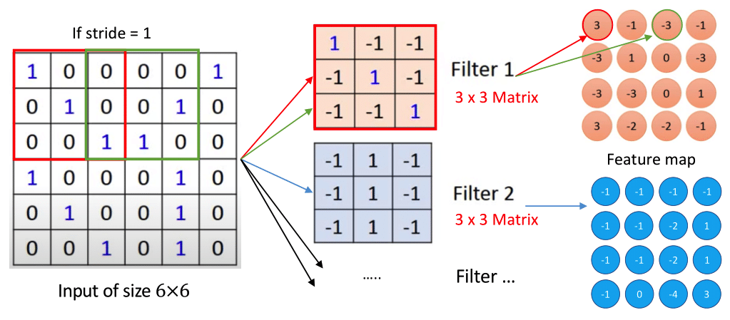
FIGURE 5.2: Basic operational structure of the convolutional layer

The input of the Neural Networks might be assumed as a \(6\times6\) matrix and each element of which can be presented as the integer ‘0’, ‘1’. As mentioned before, there is a set of learnable filters in the convolutional layer and each filter can be considered as a matrix, which is similar to a neuron in a fully-connected layer. In this instance, filters of size \(3 \times 3\) slide over with a specific stride across the entire input image, and each element of the matrix or filter serves as a parameter (weight and bias) of Neural Networks. Traditionally, these parameters are not based on the initial setting but are trained through the training data.

An activated filter of size \(3 \times 3\) has an ability to detect a pattern of the same size at some spatial position in the input. The algebraic operation explicates the transformation process from the input to the feature map.

\[ X : = \begin{pmatrix} X_{11} & X_{12} & \cdots & X_{16}\\ \\ X_{21} & X_{22} & \cdots &X_{26} \\ \\ \vdots & \vdots & \ddots & \vdots \\ \\ X_{61} & X_{62} & \cdots & X_{66} \end{pmatrix}\] where \(X\) is the input matrix of size \(6 \times 6\) as mentioned before;

\[ F : = \begin{pmatrix} w_{11} & w_{12} & w_{13}\\ \\ w_{21} & w_{22} & w_{23} \\ \\ w_{31} & w_{32} & w_{33} \end{pmatrix}\] where \(F\) denotes one filter of size \(3 \times 3\); \[ \beta : = \begin{pmatrix} w_{11} & w_{12} & \cdots & w_{16}\\ \end{pmatrix}\] where \(\beta\) is a unrolled matrix or filter; \[ A_{11} = (F \times X)_{11} : = \beta \cdot \begin{pmatrix} w_{11} & w_{12} & w_{13} & w_{21} & w_{22} & w_{23} & w_{31} & w_{32} & w_{33}\\ \end{pmatrix}^{T}\\\] Therefore, the first element of the feature map \(A_{11}\) can be calculated through the dot product operation shown above. Sequentially, the second element of the feature map is determined by the sliding dot product of filter and the succeeding input matrix with the same size after setting a specific value of stride, which can be considered as a moving distance. After the whole process, a feature map of size \(4 \times 4\) has been generated. Generally, there is more than one filter in the convolutional layer and each filter generates a feature map with the same size. The result of this convolutional layer is multiple feature maps (also referred to as activation map) and these feature maps corresponding to different filters are stacked together along the depth dimension.

Another improved convolutional layer was proposed by (Kalchbrenner, Espeholt, Simonyan, Oord, et al. (2016b)) and this kind of convolution is named Dilated convolution, in order to solve the problem that the pooling operation in the pooling layer will lose a lot of information. The critical contribution of this convolution is that the receptive field of the network will not be reduced by removing the pooling operation. In other words, the units of feature maps in the deeper hidden layer can still map a larger region of the original input. As illustrated in Figure 5.3 provided by (Oord et al. (2016)), although there is no pooling layer, the original input information is still increased as the layers are deeper.

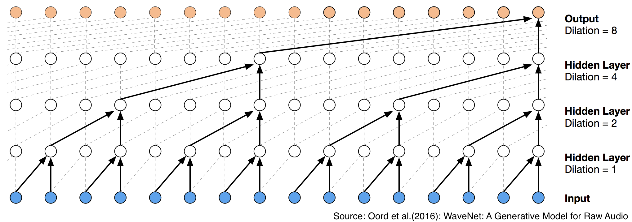
FIGURE 5.3: Visualization of dilated causal convolutional layers

5.1.2 ReLU layer

A non-linear layer (or activation layer) will be the subsequent process after each convolutional layer and the purpose of which is to introduce non-linearity to the neural networks because the operations during the convolutional layer are still linear (element-wise multiplications and summations). Generally, the major reason for introducing non-linearity is that there is a certain non-linear relationship between separate neurons. However, a convolutional layer is to perform basically a linear operation, and therefore, consecutive convolution layers are essentially equivalent to a single convolution layer, which is only used to reduce the representational power of the networks. As a result, the property of non-linearity between neurons has not been reflected and it is necessary to establish an activation function between the convolutional layer to avoid such an issue.

Activation function, which performs a non-linear transformation, plays a critical role in CNN to decide whether a neuron should be activated or ignored. Several activation functions are available after the convolutional layer, such as hyperbolic function and sigmoid function, etc., among of which ReLU is the most commonly used activation function in neural networks, especially in CNNs(Krizhevsky, Sutskever, and Hinton 2012) because of its two properties:

• Non-linearity: ReLU is the abbreviation of Rectified Linear Unit and defined mathematically as below: \[ R(z)=z^{+}= max(0,z)\]

Where z denotes the output element of the previous convolutional layer. All negative values of feature maps from the previous will be replaced by setting them to zero.

• Non-Saturation: Saturation arithmetic is a kind of arithmetic in which all operations are limited to a fixed range between a minimum and maximum value.
  • \(f\) is non-saturating iff \((|\displaystyle{\lim_{z \to -\infty}f(z)}|=+\infty) \cup (|\displaystyle{\lim_{z \to +\infty}f(z)}|=+\infty)\)
  • \(f\) is saturating iff \(f\) is not non-saturating

As illustrated in Figure 5.4, compared with saturating activation sigmoid function that saturate at large values of the input, ReLU activation function does not saturate(Krizhevsky, Sutskever, and Hinton 2012) and the gradient of it is 0 on the negative x-axis and 1 on the positive side, which is a benefit of using this activation function because the updates to the weights of the neural networks at each iteration are consistent with the gradient of the activation function. To be more specific, neuron`s weights will stop updating if its gradient is close to zero. It is obviously problematic if such a scenario appears too early in the training process.

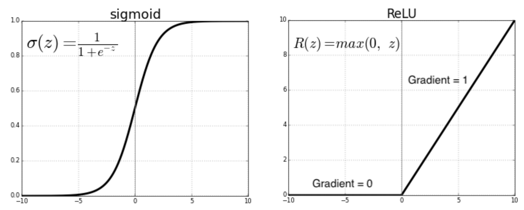
FIGURE 5.4: Comparison between saturating and non-saturating activation function

The following Figure 5.5 based on Figure 5.2 indicates a simplified version of the ReLU layer. Every single element of multiple feature maps, which is determined from the previous convolutional layer, will be further calculated by the ReLU activation function in this layer. Specifically, all positive values remain the same, and negative values are replaced by setting them to zero. The output after the ReLU layer, which has an identical network structure with the feature map from the previous convolutional layer, will be used as an input for the subsequent convolutional layer.

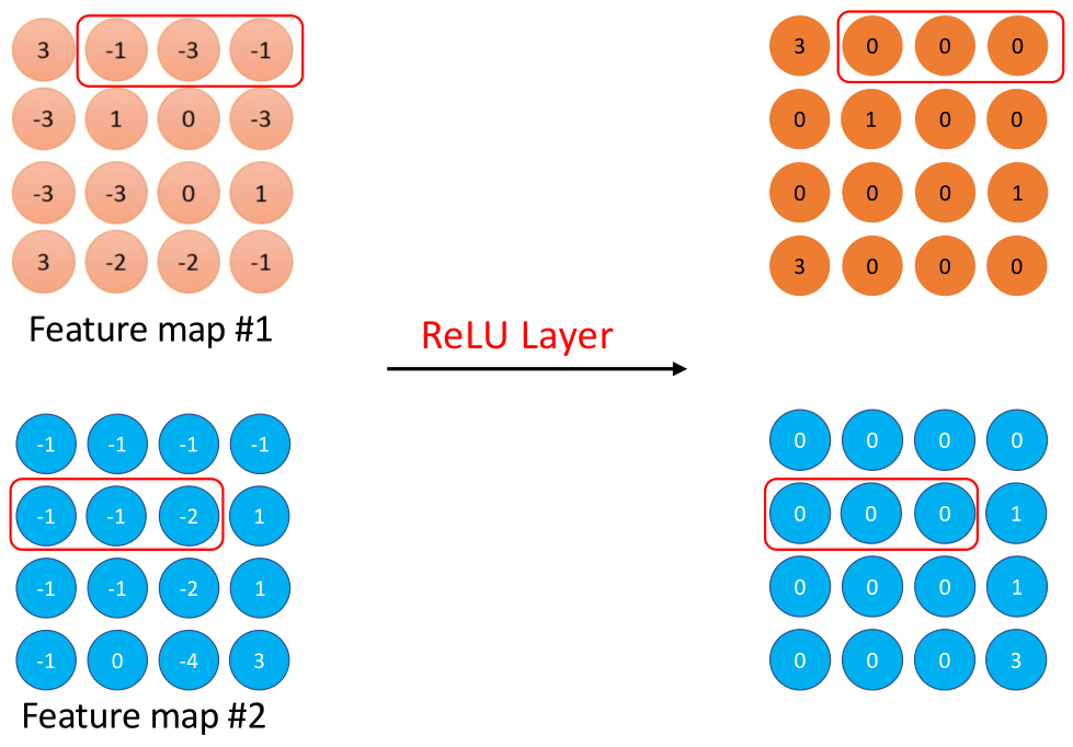
FIGURE 5.5: Basic operational structure of the ReLU layer

5.1.3 Pooling layer

The pooling layer is a concept that can be intuitively understood. The purpose of the pooling layer is to reduce progressively the spatial size of the feature map, which is generated from the previous convolutional layer, and identify important features.

There are multiple pooling operations, such as average pooling, \(l_{2}-norm\) pooling, and max pooling, Among which max pooling is the most commonly used function(Scherer, Müller, and Behnke (2010)), and the idea of max pooling is that the exact location of a feature is less important than its rough location relative to other features (Yamaguchi et al. (1990)). Simultaneously, this process helps to control overfitting to a certain extent. The following Figure 5.6 illustrates an example that constructs a basic operational structure of the max pooling.

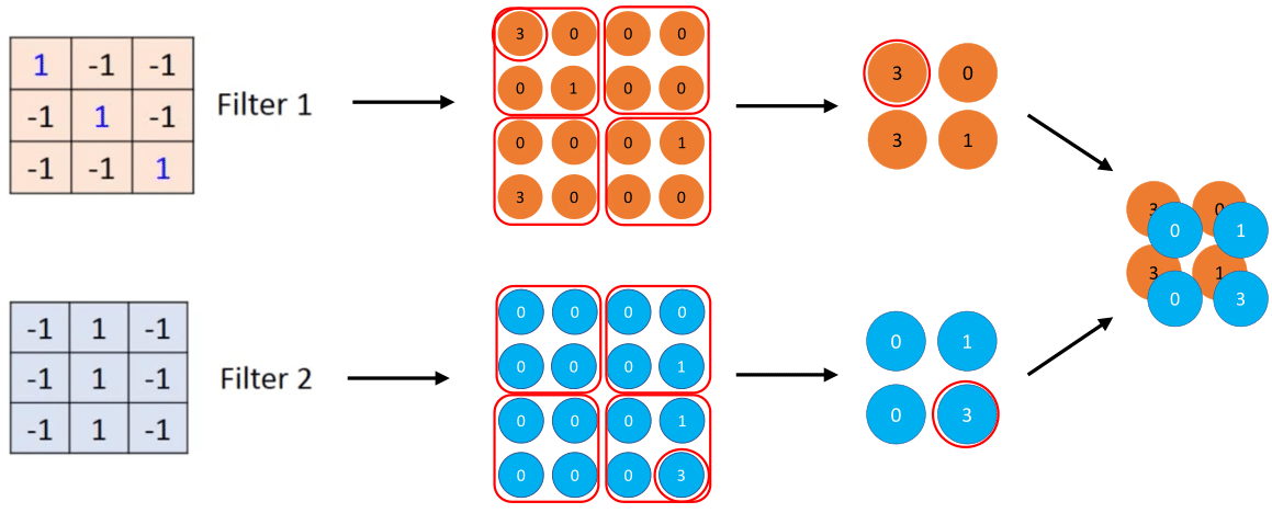
FIGURE 5.6: Basic operational structure of the max pooling layer

The example mentioned above shows that two feature maps are generated according to two different filters. In this case, these feature maps of size \(4\times4\) are separated into four non-overlapping sub-regions of size \(2\times2\), and every single sub-region is named as depth slice. The Maximum value of each sub-region will be stored in the output of the pooling layer. As a result, the input dimensions are further reduced from \(4\times4\) to \(2\times2\).

Some of the most critical reasons why adding max pooling layer to neural networks include the following:

• Reducing computation complexity: Since max pooling is reducing the dimension of the given output of a convolutional layer, the networks will be able to detect larger areas of the output. This process reduces the number of parameters in the neural networks and consequently reduces computational load.
• Controlling overfitting: Overfitting appears when the model is too complex or fits the training data too well. It may lose the true structure and then becomes difficult to generalize to new cases that are in the test data. With max-pooling operation, not all features but the primary features from each sub-region are extracted. Therefore, max-pooling operation reduces the probability of overfitting to a great extent.

Except for this most commonly applied operation in NLP, several pooling operations for different intention include the following:

• Average pooling is usually used for topic models. If a sentence has different topics and the researchers assume that max pooling extracts insufficient information, average pooling can be considered as an alternative.

• Dynamic pooling proposed by (Kalchbrenner, Grefenstette, and Blunsom (2014)) has an ability to dynamically adjust the number of features according to the network structure. More specifically, by combining the adjacent word information at the bottom and passing it gradually, new semantic information is recombined at the upper layer, so that words far away in the sentence also have interactive behavior (or some kind of semantic connection). Eventually, the most important semantic information in the sentence is extracted through the pooling layer.

5.1.4 Fully-connected layer

As we mentioned in the previous section, one or more fully-connected layers are connected after multiple convolutional layers and pooling layers, each neuron in the fully connected layer is fully connected with all the neurons from the penultimate layer. The fully-connected layer, shown in Figure 5.7, can integrate local information with class distinction in the convolutional layer or pooling layer. In order to improve the CNN network performance, the excitation function of each neuron in the fully connected layer generally uses the ReLU function.

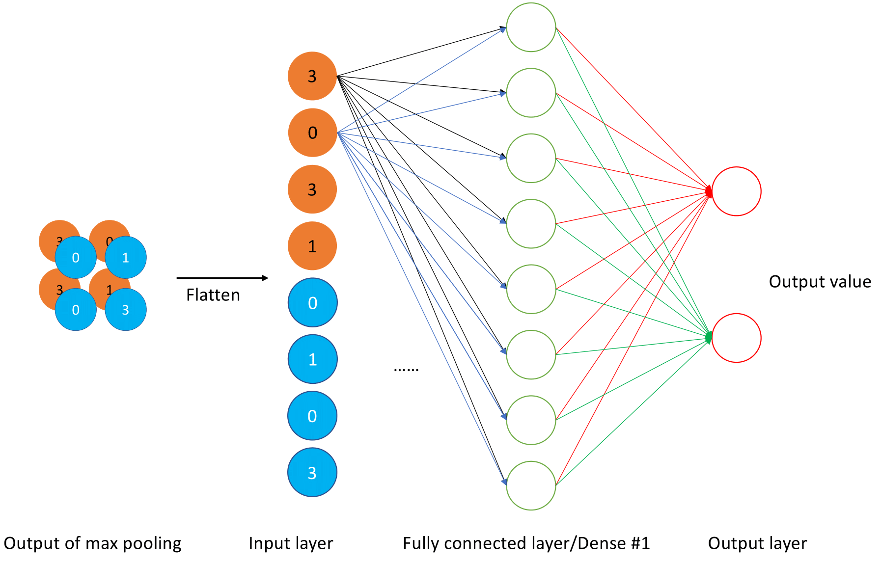
FIGURE 5.7: Basic operational structure of the fully connected layer

5.2 CNN for sentence classification

The explanation of CNN’s basic architecture provided in the first sub-chapters is based on a general example. Many researchers constructed their own specific CNN models based on this basic architecture in recent years and achieved outstanding results in the field of NLP. Therefore, this section explores four superior CNN architecture with some technical detail and their performance comparison will be provided in later sub-chapters of this report.

5.2.1 CNN-rand/CNN-static/CNN-non-static/CNN-multichannel

The first model to explore is published by (Kim (2014)), one of the highlights of this model is that the architecture is conceptually simple and efficient when dealing with the tasks of sentiment analysis and question classification. As illustrated in Figure 5.8 provided by (Kim (2014)), a simple CNN architecture of (Collobert et al. (2011)) with a single convolutional layer is utilized and the general architecture includes the following sub-structure:

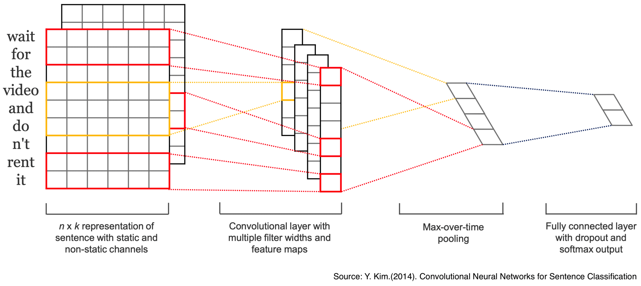
FIGURE 5.8: Model architecture of CNN for sentence classification

1. Representation of sentence: Assume that there are \(n\) words in a sentence, and each word is denoted as \(x_{i};\{i \in \mathbb{N} \mid 1 \leq i \leq n \}\) and \(x_{i} \in \mathbb{R}^{k}\) to the \(k\)-dimensional word vector. Therefore, a sentence can be represented as: \[ X_{1:n}=X_{1} \oplus X_{2} \oplus ... \oplus X_{n} \] Where \(\oplus\) is the concatenation operator.

2. Convolutional layer: Let a filter denote as \(w \in \mathbb{R}^{hk}\), which is used to a window of \(h\) words. A feature map \(c=[c_1,c_2,…,c_{n-h+1}]\) can be generated by: \[ c_i=f(w×x_{i:i+h-1}+b) \] where \(b \in \mathbb{R}\) is a bias term.

3. Max-over-time pooling: Pooling operation has been applied for the respective filter to select the most important feature from each feature map \(\hat{c} =max(\boldsymbol{c})\), notice that one feature \(\hat{c}\) is generated by one filter, and these features will be passed to the last layer.

4. Fully connected layer: The selected features \(\boldsymbol{Z}=[\hat{c}_1,\hat{c}_2,…,\hat{c}_j]\) from the previous layer have been flattened into a single vector, in order to aggregate each of them and therefore a specific class can be assigned to it based on the entire input.

CNN is a feed-forward model without cyclic connection. To be more specific, the direction of information flow in a forward model is in one direction (i.e from inputs to outputs). However, the models are trained or learned by the use of backward propagation (i.e from outputs to inputs), where the gradients are recalculated at each epoch to avoid co-adaptation.

In a forward propagation of this CNN, the output unit y based on the selected features \(\boldsymbol{Z}\) is determined by using \[y=w \cdot z+b\] In a backward propagation, a dropout mechanism is applied as follows. \[y=w \cdot (z \circ r)+b\] Where \(\circ\) is the element-wise multiplication operator and \(r \in \mathbb{R}^{m}\) denotes a ‘masking’ vector of Bernoulli random variables with probability \(p\) of being 1. As a result, gradients are backpropagated with probability \(p\) and weights \(\hat{w}\) are trained by using \[\hat{w}=pw\]

Based on the model architecture described above, four derivative CNN models are introduced by (Kim (2014)) and the major difference among them are listed below:

• CNN-rand: All words are randomly initialized and then modified during training.
• CNN-static: A model with pre-trained word vectors by using word2vec and keep them static.
• CNN-non-static: A model with pre-trained word vectors by using word2vec and these word vectors are fine-tuned for each task.
• CNN-Multichannel: A model with two channels generated by two sets of words vectors and each filter is employed to both channels.

5.2.2 Character-level ConvNets

The second model is published by (Zhang, Zhao, and LeCun (2015)), the two major differences of which compared with the previous model from (Kim (2014)) include the following:

1. The model architecture with 6 convolutional layers and 3 fully-connected layers (9 layers deep) is relatively more complex.
2. Different from the previous word-based Convolutional neural networks (ConvNets), this model is at character-level by using character quantization.

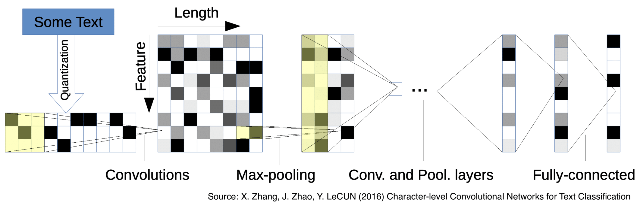
FIGURE 5.9: Model architecture of character-level CNN

The Figure 5.9 above provided by (Zhang, Zhao, and LeCun (2015)) shows the basic architecture of Character-level ConvNets, the corresponding explanation of the main components will be provided below:

1. Character quantization: The input characters will be transformed into an encoding matrix of size \(m \times l_0\) by using 1-of-\(m\) encoding (or “one-hot” encoding). To be noticed that, The length of the character exceeds the determined value \(l_0\) and will be ignored and the black characters as well as the characters that are not in the alphabet will be quantized as zero vectors.

2. Temporal convolutional module: A sequence of encoded characters followed by a temporal convolutional module, which is a variation over Convolutional Neural Networks works for sequence modelling tasks. To be more specific, when sentiment analysis is performed by using ConvNets, a fixed-size input will be a precondition, we can adjust the initial input length by truncating or padding the actual input to satisfy this criterion without affecting the sentiment and sequentially generate fixed-size outputs. Conceptually, this kind of 1-D convolution is called temporal convolution and the convolutional function defined as follow: \[h(y)=\sum_{x=1}^{k}f(x)\cdot g(y \cdot d -x+c)\] where \(h_{j}(y)\) denotes outputs of the convolutional layer; a discrete kernel functions \(f_{i,j} \in [1,k] \to \mathbb{R}\) (\((i=1,...,m\) and \(j=1,...,n)\)) is also called weights; \(d\) is denoted as stride; \(c= k-d+1\) is used as an offset constant.

3. Temporal max-pooling: Based on the research of (Boureau, Ponce, and LeCun (2010)), a 1-D version of the max-pooling \(h(y)\) is employed in this ConvNets, which is defined as

\[h(y)=max (g(y \cdot d -x+c))\] With the help of this pooling function, it is possible to train ConvNets deeper than 6 layers.

4. ReLU layer: the activation function used in this model is similar to ReLU \(h(x)=max\{0,x\}\). More specifically, the algorithm is stochastic gradient descent (SGD). However, SGD is influenced by the strong curvature of the optimization function and moves slowly towards the minimum. Therefore, based on the research of Sutskever et al. (2013), a momentum of 0.9 and an initial step size 0.01 are established to reach the minimum more quickly.

5.2.3 Very Deep CNN

The third character-level model to explore is from Schwenk et al. (2017). Inspired by (Simonyan and Zisserman (2015)), a CNN model with deep architectures of many convolutional layers is developed, the significant difference of which from the previous model architecture is that this model applies much deeper architectures (i.e. using up to 29 convolutional layers), in order to learn hierarchical representations of whole sentences. The overall architecture will be explored based on Figure 5.10 and 5.11 also provided by (Schwenk et al. (2017)).

FIGURE 5.10: Architecture of convolutional block

The above Figure 5.10 shows an architecture of a convolutional block with 256 feature maps and the kernel size of all the convolutions is 3. The convolutional block is composed of two consecutive convolutional layers, and each one followed by a temporal BatchNorm layer (Ioffe and Szegedy (2015)) and a ReLU activation.

Batch normalization, as the name suggests, is a normalized operation commonly used to improve the speed and stability of neural networks, especially for the deep neural network. The following shows the algorithm of Batch Normalizing Transform.

For a layer with \(d\)-dimensional input \(x = (x^{(1)},...,x^{(d)})\)

1. \(\mu_B = \frac 1 m \sum_{i=1}^m x_i\) //mini-batch mean

2. \(\sigma_B^2 = \frac 1 m \sum_{i=1}^m (x_i-\mu_B)^2\) // mini-batch variance

3. \(\hat{x}_{i}^{(k)} = \frac {x_i^{(k)}-\mu_B^{(k)}}{\sqrt{\sigma_B^{(k)^2}+\epsilon}}\) // normalize

where \(k \in [1,d]\) and \(i \in [1,m]\); \(\mu_B^{(k)}\)and \(\sigma_B^{(k)^2}\) are the per-dimension mean and variance; \(\epsilon\) is an arbitrarily small constant.

4. \(y_i^{(k)} = \gamma^{(k)} \hat{x}_{i}^{(k)} +\beta^{(k)}\) // scale and shift

where the parameters \(\gamma^{(k)}\)and \(\beta^{(k)}\) are subsequently learned in the optimization process.

To be more specific, in the SGD training process, use mini-batch to normalize the corresponding activation so that the mean value of the results (all dimensions of the output signal) is \(0\) and the variance is \(1\). Subsequently, two independent learnable parameters \(\beta\) and \(\gamma\) will be introduced in the final operation “scale and shift”.

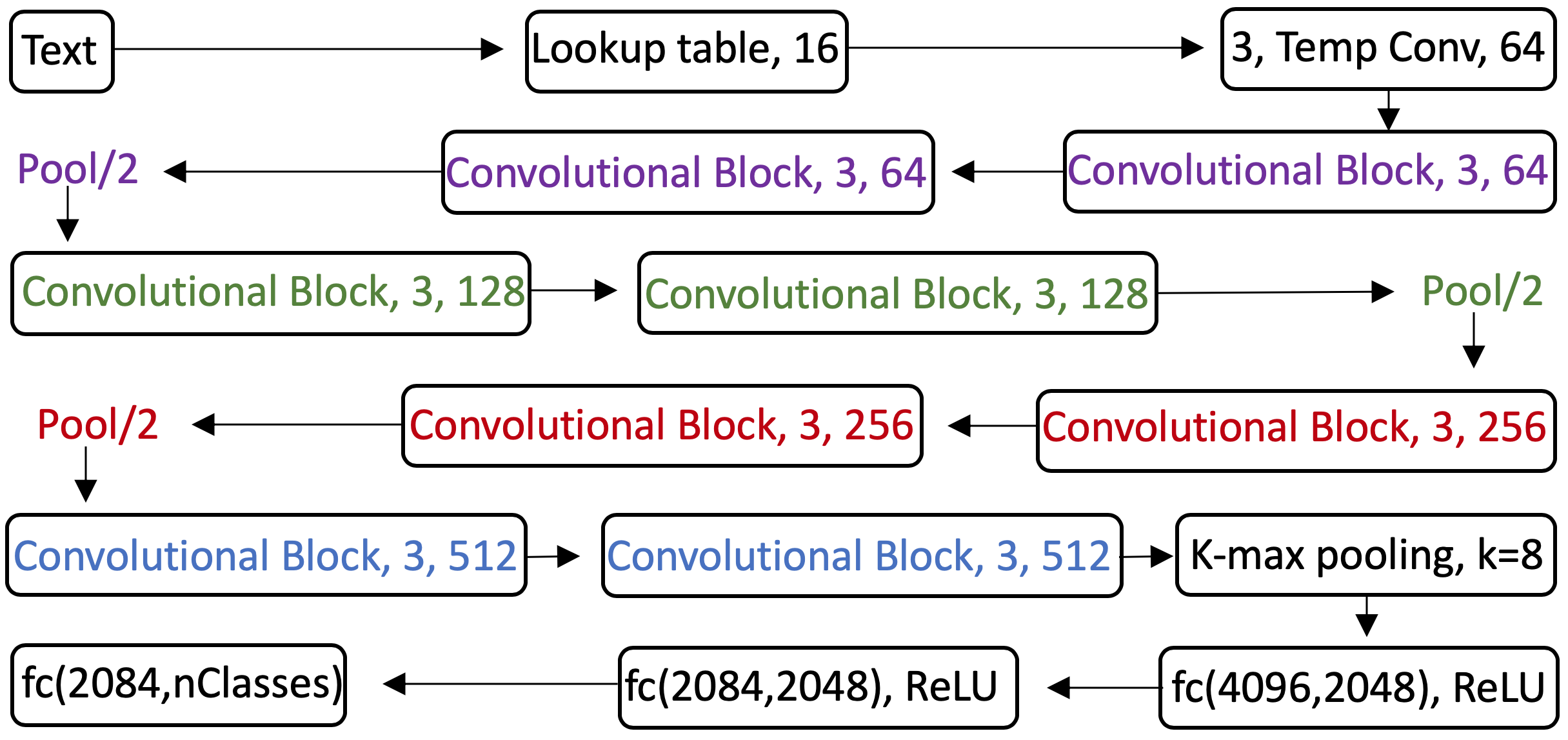
FIGURE 5.11: Very Deep Convolutional Networks architecture

The overall architecture of VDCNN is shown in Figure 5.11 above, The first layer contains 64 convolutions of size 3 after importing the initial text, a series of convolutional blocks are connected after the convolutional layer, and the number of feature maps is determined by two rules:

1. If the temporal resolution of output remains the same，the layers have the same number of feature maps.
2. If the temporal resolution is halved, the number of feature maps is doubled.

Based on the above rules, the size of resolution will be halved after each pooling operation, so the number of feature maps will be corresponding to double from 128 to 512.

k-max pooling: The result of k-max pooling is not to return a single maximum value, but to return k sets of maximum values, which are a subsequence of the original input. The parameter \(k\) in the pooling can be a dynamic function, and this specific value depends on the input or other parameters of the network. the specific dynamic function is as follows.

\[k_{l}=max(k_{top},\lceil \frac{L-l}{L}s \rceil)\] In this formula, \(s\) denotes the length of the sentence, \(L\) represents the total number of convolutional layers, and \(l\) represents the number of convolutional layers that are currently in. so it can be seen that \(k\) varies with the length of the sentence and the depth of the network change. The advantage of K-max pooling is that it not only extracts more than one important information in the sentence but also retains their order.

The output of k-max pooling is transformed into a single vector which will be used as input to a three fully-connected layer with ReLU activation function and softmax outputs.

5.2.4 Deep Pyramid CNN

The last model we will discuss in this chapter is Deep Pyramid Convolutional Neural Networks (DPCNN), which is published by (Johnson and Zhang (2017)). The major difference from the previous deep CNN is that this model is constructed of a low-complexity word-level deep CNN architecture. The motivation for using such an architecture based on the point of view of (Johnson and Zhang (2017)) includes the following:

low-complexity: As the research of (Johnson and Zhang (2016)) shows that very shallow 1-layer word-level CNNs such as (Kim (2014)) performs more accurate and much faster than the deep character-level CNNs of (Schwenk et al. (2017)).

word-level: word-level CNNs are more accurate and much faster than the state-of-the-art very deep networks such as character-level CNNs even in the setting of large training data.

The description of key features of DPCNN will be provided based on the Figure 5.12 from (Johnson and Zhang (2017)) as follows.

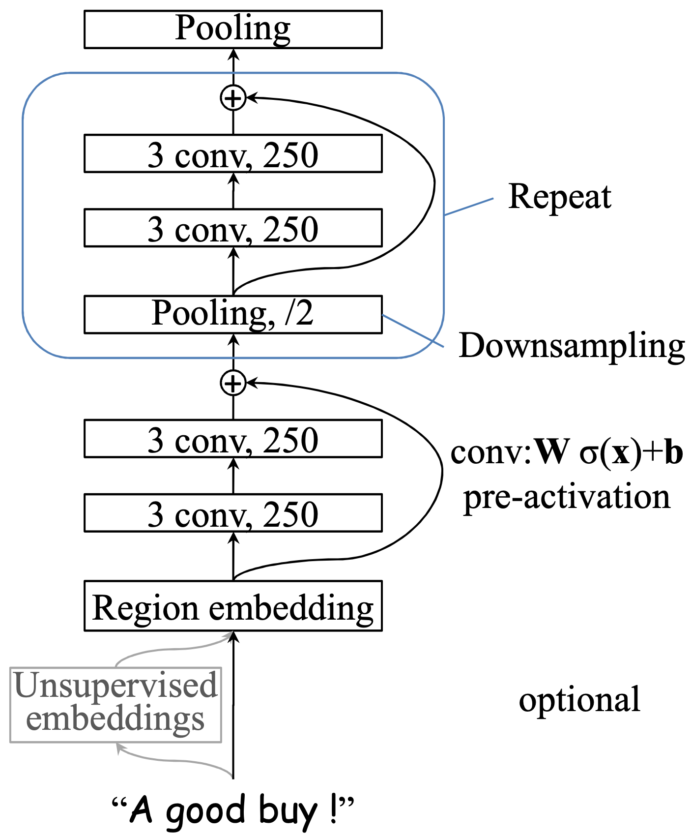
FIGURE 5.12: Architecture of Deep Pyramid CNN

Text region embedding with unsupervised embeddings: This technique is based on the basic region embedding. More specifically, the embedding generated after performing a set of convolution operations on different sizes of text area/segment (such as bi-grams or tri-grams) and these convolution operations are achieved by using multi-size learnable convolutional filters. There are two options when performing convolution operation on a text area, For example, by using tri-grams, one is to preserve the word order, which means that setting a set of 2D convolution kernels with size= \(3 \times D\) to convolve the 3 words (where D is the word embedding dimension), another is not to preserve the word order (i.e. using the Bag-of-words model). Preliminary experiments indicated that considering word order does not significantly help to improve accuracy and increase computational complexity. Therefore, DPCNN adopts a method similar to the Bag-of-words model. In addition to this, to avoid the overfitting caused by high representation power of n-gram, a technique called tv-embedding (two-views embedding) will be introduced in DPCNN, which means that a region of text as view-1 and its adjacent regions as view-2 will be pre-defined, and view-1 will be trained to predict view-2 in one hidden layer and it will be considered as input, this process is called unsupervised embedding.

Shortcut connections with pre-activation : From experience, the depth of the network is critical to the performance of the model，Because by giving the model more parameters, the model can fit the train data at least as well as before and detect more complex feature patterns. However, the experimental results show that the training accuracy will decrease as the depth of the network increases, the reason is Degradation problem or so-called vanishing/exploding gradients. More specifically, Assume we consider a shallow architecture and add more layers linked by identity mapping (i.e. \(f(z) = z\)). The value of the output after multiple nonlinear layers should also be z, but the result will be biased due to the existence of this Degradation problem. Therefore, the shortcut connections were proposed by (He et al. (2016a)). Formally, denoting the desired underlying mapping as \(H(z)\), \(f(z) := H(z)−z\) is denoted as a residual function, so the original mapping is recast into \(f(z)+z\). This technique is used to solve the problem of depth model accuracy.

Downsampling with the number of feature maps fixed: Similar to the VDCNN described in the previous sub-chapter is that multiple convolutional blocks are also introduced to the architecture of DPCNN. However, the difference is that the number of feature maps is fixed instead of increasing like VDCNN, because (Johnson and Zhang (2017)) thinks increasing the number of feature maps will lead to increased computation time substantially without accuracy improvement, Therefore, the computation time and sample size for each convolution layer are halved (Downsampling).

5.3 Datasets and Experimental Evaluation

A brief description of the eight data sets will be provided in this sub-chapter, based on which the performance comparison of all four models mentioned above will also be listed.

5.3.1 Datasets

The comparison results of all CNN models explored in this chapter are based on the eight datasets complied by (Zhang, Zhao, and LeCun (2015)), summarized in the following table.

Data	AG	Sogou	Dbpedia	Yelp.p	Yelp.f	Yahoo	Ama.f	Ama.p
# of training documents	120K	450K	560K	560K	650K	1.4M	3M	3.6M
# of test documents	7.6K	60K	70K	38K	50K	60K	650K	400K
# of classes	4	5	14	2	5	10	5	2
Average #words	45	578	55	153	155	112	93	91

Based on the description of the datasets of (Johnson and Zhang (2017)), AG and Sogou are news. Dbpedia is an ontology. Yahoo consists of questions and answers from the ‘Yahoo! Answers’ website. Yelp and Amazon (‘Ama’) are reviews where .p (polarity) in the names indicates that labels are binary (positive/negative), and .f (full) indicates that labels are the number of stars. Sogou is in Romanized Chinese, and the others are in English. Classes are balanced on all the datasets. Furthermore, These eight datasets can be subdivided into two groups, the first four datasets are relatively smaller datasets and the rest of them can be classified as relatively larger data sets.

5.3.2 Experimental Evaluation

The following table provided by (Johnson and Zhang (2017)) shows the error rates in percentage on datasets described in the previous sub-chapter in comparison with all models. To be more specific, a lower error rate represents better model performance and the corresponding best results are marked in bold. tv stands for tv-embeddings. w2v stands for word2vec. (w2v) indicates that the best results among those with and without word2vec pretraining are shown. Note that best next to the model name is denoted as the model by choosing the best test error rate among several variations presented in the respective papers.

Models	Deep	Unsup. embed.	AG	Sogou	Dbpedia	Yelp.p	Yelp.f	Yahoo	Ama.f	Ama.p
DPCNN + unsupervised embed.(Johnson and Zhang (2017))	\(\surd\)	tv	6.87	1.84	0.88	2.64	30.58	23.90	34.81	3.32
ShallowCNN + unsup. embed.(Kim (2014))		tv	6.57	1.89	0.84	2.90	32.39	24.85	36.24	3.79
Very Deep char-level CNN: best (Schwenk et al. (2017))	\(\surd\)		8.67	3.18	1.29	4.28	35.28	26.57	37.00	4.28
fastText bigrams (Joulin et al. (2017))			7.5	3.2	1.4	4.3	36.1	27.7	39.8	5.4
[ZZL15]’s char-level CNN: best(Zhang, Zhao, and LeCun (2015))	\(\surd\)		9.51	4.88	1.55	4.88	37.95	28.80	40.43	4.93
[ZZL15]’s word-level CNN : best(Zhang, Zhao, and LeCun (2015))	\(\surd\)	(w2v)	8.55	4.39	1.37	4.60	39.58	28.84	42.39	5.51
[ZZL15]’s linear model: best(Zhang, Zhao, and LeCun (2015))			7.64	2.81	1.31	4.36	40.14	28.96	44.74	7.98

Based on the comparison results shown above, some of the significant results include the following:

1. DPCNN achieves an outstanding performance, which shows the lowest error rate in six of the eight datasets.

2. Shallow CNN, which possesses the simplest model architecture with only one convolutional layer, performs even better than other deep models.

3. By mere comparison of character-level CNN (Zhang, Zhao, and LeCun (2015)) and word-level CNN (Zhang, Zhao, and LeCun (2015)), the result will be that words-level CNN performs better in the smaller datasets and character-level CNN performs better in the bigger datasets.

5.4 Conclusion and Discussion

In summary, this chapter introduces the architecture of multiple CNN models and compares the performance of these models in the application of NLP especially for text categorization in different scale datasets. Subsequently, we will discuss the results obtained from the previous table in two ways including a comparison between the character-level approach and the word-level approach and depth of the model.

1. Character-level and word-level Extending from the experimental studies and the corresponding comparison results shown in the previous sub-chapter, word-level CNN possesses higher accuracy presented in lower error rate in comparison of character-level CNNs in general, although character-level CNN holds an advantage in not having to deal with millions of distinct words, word-level approach displays higher accuracy than character-level because the advantage of word-level is that Word can represent the meaning.

2. Deep and shallow model architecture DPCNN, which shows the best test error rate among all CNN models discussed in this chapter, could be considered as a kind of deeper Shallow CNN. Consequently, increasing the depth of the model can lead to an increase in parameters and increased capacity to handle complex feature patterns. Better performance of DPCNN compared with Shallow CNN evidence that increasing depth can improve accuracy to a certain extent. However, it comes to the opposite conclusion by comparing with Very Deep CNN since the probability of potential issues such as vanishing/exploding gradients will increase as the number of layers increases. Therefore, it is essential to improve the accuracy of complex and deep models by introducing appropriate components (e.g. shortcut connections).

References

Boureau, Y-Lan, Jean Ponce, and Yann LeCun. 2010. A Theoretical Analysis of Feature Pooling in Visual Recognition. https://www.di.ens.fr/willow/pdfs/icml2010b.pdf.

Collobert, Ronan, Jason Weston, Léon Bottou, Michael Karlen, Koray Kavukcuoglu, and Pavel P. Kuksa. 2011. Natural Language Processing (Almost) from Scratch. J. Mach. Learn. Res. Vol. 12. http://www.jmlr.org/papers/volume12/collobert11a/collobert11a.pdf.

He, Kaiming, Xiangyu Zhang, Shaoqing Ren, and Jian Sun. 2016a. “Deep Residual Learning for Image Recognition.” 2016 IEEE Conference on Computer Vision and Pattern Recognition (CVPR), 770–78. https://arxiv.org/pdf/1512.03385v1.pdf.

Ioffe, Sergey, and Christian Szegedy. 2015. “Batch Normalization: Accelerating Deep Network Training by Reducing Internal Covariate Shift.” ArXiv abs/1502.03167. https://arxiv.org/pdf/1502.03167.pdf.

Johnson, Rie, and Tong Zhang. 2016. “Convolutional Neural Networks for Text Categorization: Shallow Word-Level Vs. Deep Character-Level.” ArXiv abs/1609.00718. https://arxiv.org/pdf/1609.00718.pdf.

Johnson, Rie, and Tong Zhang. 2017. “Deep Pyramid Convolutional Neural Networks for Text Categorization.” In ACL. https://pdfs.semanticscholar.org/2f79/66bd3bc7aaf64c7db40fb7f3309f5207cbf7.pdf.

Joulin, Armand, Edouard Grave, Piotr Bojanowski, and Tomas Mikolov. 2017. “Bag of Tricks for Efficient Text Classification.” ArXiv abs/1607.01759. https://arxiv.org/pdf/1607.01759.pdf.

Kalchbrenner, Nal, Lasse Espeholt, Karen Simonyan, Aäron van den Oord, Alex Graves, and Koray Kavukcuoglu. 2016b. “Neural Machine Translation in Linear Time.” ArXiv abs/1610.10099. https://arxiv.org/pdf/1610.10099.pdf.

Kalchbrenner, Nal, Edward Grefenstette, and Phil Blunsom. 2014. A Convolutional Neural Network for Modelling Sentences. ArXiv. Vol. abs/1404.2188. http://mirror.aclweb.org/acl2014/P14-1/pdf/P14-1062.pdf.

Kim, Yoon. 2014. Convolutional Neural Networks for Sentence Classification. https://www.aclweb.org/anthology/D14-1181.pdf.

Krizhevsky, Alex, Ilya Sutskever, and Geoffrey E. Hinton. 2012. ImageNet Classification with Deep Convolutional Neural Networks. http://www.cs.toronto.edu/~hinton/absps/imagenet.pdf.

Oord, Aäron van den, Sander Dieleman, Heiga Zen, Karen Simonyan, Oriol Vinyals, Alex Graves, Nal Kalchbrenner, Andrew W. Senior, and Koray Kavukcuoglu. 2016. WaveNet: A Generative Model for Raw Audio. ArXiv. Vol. abs/1609.03499. https://arxiv.org/pdf/1609.03499.pdf.

Scherer, Dominik, Andreas C. Müller, and Sven Behnke. 2010. “Evaluation of Pooling Operations in Convolutional Architectures for Object Recognition.” In ICANN. http://ais.uni-bonn.de/papers/icann2010_maxpool.pdf.

Schwenk, Holger, Loïc Barrault, Alexis Conneau, and Yann LeCun. 2017. Very Deep Convolutional Networks for Text Classification. https://www.aclweb.org/anthology/E17-1104.pdf.

Simonyan, Karen, and Andrew Zisserman. 2015. “Very Deep Convolutional Networks for Large-Scale Image Recognition.” CoRR abs/1409.1556. https://arxiv.org/pdf/1409.1556.pdf.

Sutskever, Ilya, James Martens, George E. Dahl, and Geoffrey E. Hinton. 2013. “On the Importance of Initialization and Momentum in Deep Learning.” In ICML.

Yamaguchi, Kouichi, Kenji Sakamoto, Toshio Akabane, and Yoshiji Fujimoto. 1990. A Neural Network for Speaker-Independent Isolated Word Recognition. https://www.isca-speech.org/archive/archive_papers/icslp_1990/i90_1077.pdf.

Zhang, Xiang, Junbo Jake Zhao, and Yann LeCun. 2015. Character-Level Convolutional Networks for Text Classification. https://papers.nips.cc/paper/5782-character-level-convolutional-networks-for-text-classification.pdf.