Chapter 8 Attention and Self-Attention for NLP

Authors: Joshua Wagner

Supervisor: Matthias Aßenmacher

Attention and Self-Attention models were some of the most influential developments in NLP. The first part of this chapter is an overview of attention and different attention mechanisms. The second part focuses on self-attention which enabled the commonly used models for transfer learning that are used today. The final part of the chapter discusses the developments made with Self-Attention and the most common transfer learning architecture today, the Transformer.

8.1 Attention

In this part of the chapter, we revisit the Encoder-Decoder architecture that was introduced in chapter 3. We focus on the improvements that were made with the development of attention mechanisms on the example of neural machine translation (NMT).

As seen in chapter 3, vanilla Encoder-Decoder architecture passes only the last hidden state from the encoder to the decoder. This leads to the problem that information has to be compressed into a fixed length vector and information can be lost in this compression. Especially information found early in the sequence tends to be “forgotten” after the entire sequence is processed. The addition of bi-directional layers remedies this by processing the input in reversed order. While this helps for shorter sequences, the problem still persists for long input sequences. The development of attention enables the decoder to attend to the whole sequence and thus use the context of the entire sequence during the decoding step.

8.1.1 Bahdanau-Attention

In 2014, Bahdanau, Cho, and Bengio (2014) proposed attention to fix the information problem that the early encoder-decoder architecture faced. Decoders without attention are trained to predict \(y_{t}\) given a fixed length context vector \(c\) and all earlier predicted words \(\{y_t, \dots, y_{t-1}\}\). The fixed length context vector is computed with \[c=q(\{h_1,\dots,h_T\})\] where \(h_1,\dots,h_T\) are the the hidden states of the encoder for the input sequence \(x_1,\dots, x_T\) and \(q\) is a non-linear function. Sutskever, Vinyals, and Le (2014) for example used \(c = q(\{h_1,\dots,h_T\}) = h_T\) as their non-linear transformation which remains a popular choice for architectures without attention. It is also commonly used for the initialisation of the decoder hidden states.

Attention changes the context vector \(c\) that a decoder uses for translation from a fixed length vector \(c\) of a sequence of hidden states \(h_1, \dots, h_T\) to a sequence of context vectors \(c_i\). The hidden state \(h_i\) has a strong focus on the i-th word in the input sequence and its surroundings. If a bi-directional encoder is used, each \(h_i\) is computed by a concatenation of the forward \(\overrightarrow{h_i}\) and backward \(\overleftarrow{h_i}\) hidden states:

\[ h_i = [\overrightarrow{h_i}; \overleftarrow{h_i}], i = 1,\dots,n \] These new variable context vectors \(c_i\) are used for the computation of the decoder hidden state \(s_t\). At time-point \(t\) it is computed as \(s_t = f(s_{t-1},y_{t-1},c_t)\) where \(f\) is the function resulting from the use of a LSTM- or GRU-cell. The context vector \(c_t\) is computed as a weighted sum of the hidden states \(h_1,\dots, h_{T_x}\):

\[ c_t = \sum^{T_x}_{i=1}\alpha_{t,i}h_i. \] Each hidden state \(h_i\) is weighted by a \(\alpha_{t,i}\). The weight \(\alpha_{t,i}\) for each hidden state \(h_i\) is also called the alignment score. These alignment scores are computed as:

\[ \alpha_{t,i} = align(y_t, x_i) =\frac{exp(score(s_{t-1},h_i))}{\sum^{n}_{i'=1}exp(score(s_{t-1},h_{i'}))} \] with \(s_{t-1}\) being the hidden state of the decoder at time-step \(t-1\). The alignment score \(\alpha_{t,i}\) models how well input \(x_i\) and output \(y_t\) match and assigns the weight to \(h_i\). Bahdanau, Cho, and Bengio (2014) parametrize their alignment score with a single-hidden-layer feed-forward neural network which is jointly trained with the other parts of the architecture. The score function used by Bahdanau et al. is given as

\[ score(s_t,h_i) = v_\alpha^Ttanh(\mathbf{W}_\alpha[s_t;h_i]) \] were tanh is used as a non-linear activation function and \(v_\alpha\) and \(W_\alpha\) are the weight matrices to be learned by the alignment model. The alignment score function is called “concat” in Luong, Pham, and Manning (2015) and “additive attention” in Vaswani et al. (2017) because \(s_t\) and \(h_i\) are concatenated just like the forward and backward hidden states seen above. The attention model proposed by Bahdanau et al. is also called a global attention model as it attends to every input in the sequence. Another name for Bahdanaus attention model is soft attention because the attention is spread thinly/weakly/softly over the input and does not have an inherent hard focus on specific inputs. A nice by-product of attention mechanisms is the matrix of alignment scores which can be visualised to show the correlation between source and target words as seen in 8.1.

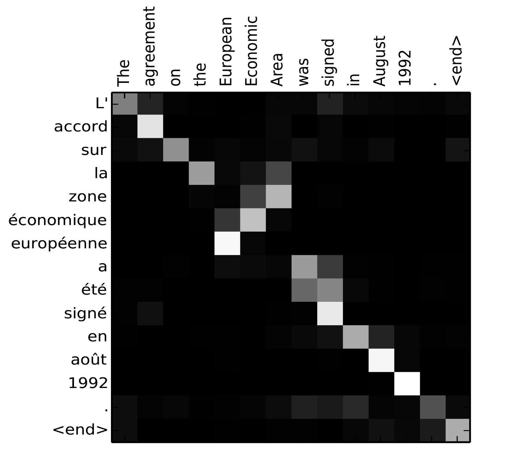
FIGURE 8.1: Alignment Matrix visualised for a French to English translation. White squares indicate high aligment weights between input and output. Image source: Fig 3 in (Bahdanau, Cho, and Bengio 2014)

8.1.2 Luong-Attention

While Bahdanau, Cho, and Bengio (2014) were the first to use attention in neural machine translation, Luong, Pham, and Manning (2015) were the first to explore different attention mechanisms and their impact on NMT. Luong et al. also generalise the attention mechanism for the decoder which enables a quick switch between different attention functions. Bahdanau et al. only consider

\[ score(s_t,h_i) = v_\alpha^Ttanh(\mathbf{W}_\alpha[s_t;h_i]), \] while Luong et al. additionally introduce a general, a location-based and a dot-product score function for the global attention mechanism as described in table 8.1.

Score-function	Name
\(\text{score}(\boldsymbol{s}_t, \boldsymbol{h}_i) = \boldsymbol{s}_t^\top\mathbf{W}_a\boldsymbol{h}_i\)	General
\(\alpha_{t,i} = \text{softmax}(\mathbf{W}_a \boldsymbol{s}_t)\)	Location-based
\(\text{score}(\boldsymbol{s}_t, \boldsymbol{h}_i) = \boldsymbol{s}_t^\top\boldsymbol{h}_i\)	Dot-product

Table 8.1: (#tab:luong-score-functions) Different score function proposed by Luong et al.

As Luong, Pham, and Manning (2015) don’t use a bidirectional encoder, they simplify the hidden state of the encoder from a concatenation of both forward and backward hidden states to only the hidden state at the top layer of both encoder and decoder.

The attention mechanisms seen above attend to the entire input sequence. While this fixes the problem of forgetful sequential models discussed in the beginning of the chapter, it also has the drawback that it is expensive and can potentially be impractical for long sequences e.g. the translation of entire paragraphs or documents. These problems encountered with global or soft attention mechanisms can be mitigated with a local or hard attention approach. While it was used by Xu et al. (2015) for caption generation of images with a CNN and by Gregor et al. (2015) for the generation of images, the first application and differentiable version for NMT is from Luong, Pham, and Manning (2015).

Different from the global attention mechanism, the local attention mechanism at timestep \(t\) first generates an aligned position \(p_t\). The context vector is then computed as a weighted average over only the set of hidden states in a window \([p_t-D,p_t+D]\) with \(D\) being an empirically selected parameter. This constrains the above introduced computation for the context vector to:

\[ c_t = \sum^{p_t+D}_{i=p_t-D}\alpha_{t,i}h_i. \]

The parts outside of a sentence are ignored if the window crosses sentence boundaries. The computation of the context vector changes compared to the global model which can be seen in Figure 8.2.

FIGURE 8.2: Global and local attention illustrated. Encoder in blue, Decoder in red. \(\overline{h}_s\) and \(h_t\) in the image correspond to \(h_t\) and \(s_t\) in the previous text. Additional computations and differences to previous described architecture is found in the next sub-chapter. Image source: Fig. 2 and 3 in (Luong, Pham, and Manning 2015)

Luong et al. introduce two different concepts for the computation of the alignment position \(p_t\).

The first is the monotonic alignment(local-m). This approach sets \(p_t= t\) with the assumption that both input and output sequences are roughly monotonically aligned.

The other approach, predictive alignment (local-p), predicts the aligned position with: \[ p_t = S \cdot sigmoid(v_p^\top tanh(W_ph_t)) \] where \(W_p\) and \(v_p\) are the parameters that are trained to predict the position. \(S\) is the length of the input sentence which leads, with the additional sigmoid function, to \(p_t \in [0,S]\). A Gaussian distribution centred around \(p_t\) is placed by Luong, Pham, and Manning (2015) to favour alignment points closer to \(p_t\). This changes the alignment weights to: \[ \alpha_{t,i} = align(y_t, x_i)exp(-\frac{(i-p_t)^2}{2\sigma^2}) \] where the standard deviation is empirically set to \(\sigma = \frac{D}{2}\). This utilization of \(p_t\) to compute \(\alpha_{t,i}\) allows the computation of backpropagation gradients for \(W_p\) and \(v_p\) and is thus ``differentiable almost everywhere’’ Luong, Pham, and Manning (2015) while being less computationally expensive than global attention.

8.1.3 Computational Difference between Luong- and Bahdanau-Attention

As previously mentioned, Luong et al. not only introduced different score functions in addition to Bahdanau et al.’s concatenation/additive score function, they also generalized the computation for the context vector \(c_t\). In Bahdanau’s version the attention mechanism computes the variable length context vector first which is then used as input for the decoder. This necessitates the use of the last decoder hidden state \(s_{t-1}\) as input for the computation of the context vector \(c_t\):

\[ \alpha_{t,i} = align(y_t, x_i) =\frac{exp(score(s_{t-1},h_i))}{\sum^{n}_{i'=1}exp(score(s_{t-1},h_{i'}))} \]

Luong et al. compute their context vector with the current decoder hidden state \(s_t\) and modify the decoder output with the context vector before it is processed by the last softmax layer. This allows for easier implementation of different score functions for the same attention mechanism. Implementations of both vary e.g. this version of Bahdanau attention in Pytorch concatenates the context back in after the GRU while this version for an NMT model with Bahdanau attention does not. Readers that are trying to avoid a headache can build upon this version from Tensorflow which uses the AttentionWrapper function which handles the specifics of the implementation.

An illustration of a reduced version of the two different attention concepts can be found in Figure 8.3.

FIGURE 8.3: Bahdanau and Luong attention mechanisms illustrated. The attention layer is bounded in the red box. Orange denotes inputs, outputs and weights. Blue boxes are layers. Green boxes denote operations e.g. softmax or concatenation([x;y]).

8.1.4 Attention Models

Attention was in the beginning not directly developed for RNNs or even NLP. Attention was first introduced in Graves, Wayne, and Danihelka (2014) with a content-based attention mechanism (\(\text{score}(\boldsymbol{s}_t, \boldsymbol{h}_i) = \text{cosine}[\boldsymbol{s}_t, \boldsymbol{h}_i]\)) for Neural Turing Machines. Their application for NLP related tasks were later developed by Luong, Pham, and Manning (2015), Bahdanau, Cho, and Bengio (2014) and Xu et al. (2015). Xu et al. (2015) were the first publication to differentiate between soft/global and hard/local attention mechanisms and did this in the context of Neural Image Caption with both mechanisms being close to what was used by Luong et al. in the previous section. Cheng, Dong, and Lapata (2016) were the first to introduce the concept of self-attention, the third big category of attention mechanisms.

8.2 Self-Attention

Cheng, Dong, and Lapata (2016) implement self-attention with a modified LSTM unit, the Long Short-Term Memory-Network (LSTMN). The LSTMN replaces the memory cell with a memory network to enable the storage of ``contextual representation of each input token with a unique memory slot and the size of the memory grows with time until an upper bound of the memory span is reached’’ Cheng, Dong, and Lapata (2016). Self-Attention, as the name implies, allows an encoder to attend to other parts of the input during processing as seen in Figure 8.4.

FIGURE 8.4: Illustration of the self-attention mechanism. Red indicates the currently fixated word, Blue represents the memories of previous words. Shading indicates the degree of memory activation. Image source: Fig. 1 in (Cheng, Dong, and Lapata 2016).

While the LSTMN introduced self-attention, it retains the drawbacks that come from the use of a RNN which are discussed at the end of the Transformer section. Vaswani et al. (2017) propose the Transformer architecture which uses self-attention extensively to circumvent these drawbacks.

8.2.1 The Transformer

RNNs were, prior to Transformers, the state-of-the-art model for machine translation, language modelling and other NLP tasks. But the sequential nature of a RNN precludes parallelization within training examples. This becomes critical at longer sequence lengths as memory constraints limit batching across examples. While much has been done to minimize these problems, they are inherent in the architecture and thus still remain. An attention mechanism allows the modelling of dependencies without regard for the distance in either input or output sequences. Most attention mechanisms, as seen in the previous sections of this chapter, use recurrent neural networks. This limits their usefulness for transfer learning because of the previously mentioned constraints that recurrent networks have. Models like ByteNet from Kalchbrenner, Espeholt, Simonyan, Oord, et al. (2016a) and ConvS2S from Gehring et al. (2017) alleviate the problem with sequential models by using convolutional neural networks as basic building blocks. ConvS2S has a linear increase in number of operations to relate signals from two arbitrary input or output positions with growing distance. ByteNet has a logarithmical increase in number of operations needed. The Transformer architecture from Vaswani et al. (2017) achieves the relation of two signals with arbitrary positions in input or output with a constant number of operations. It was also the first model that relied entirely on self-attention for the computation of representations of input or output without using sequence-aligned recurrent networks or convolutions.

While the Transformer architecture doesn’t use recurrent or convolutional networks, it retains the popular encoder-decoder architecture.

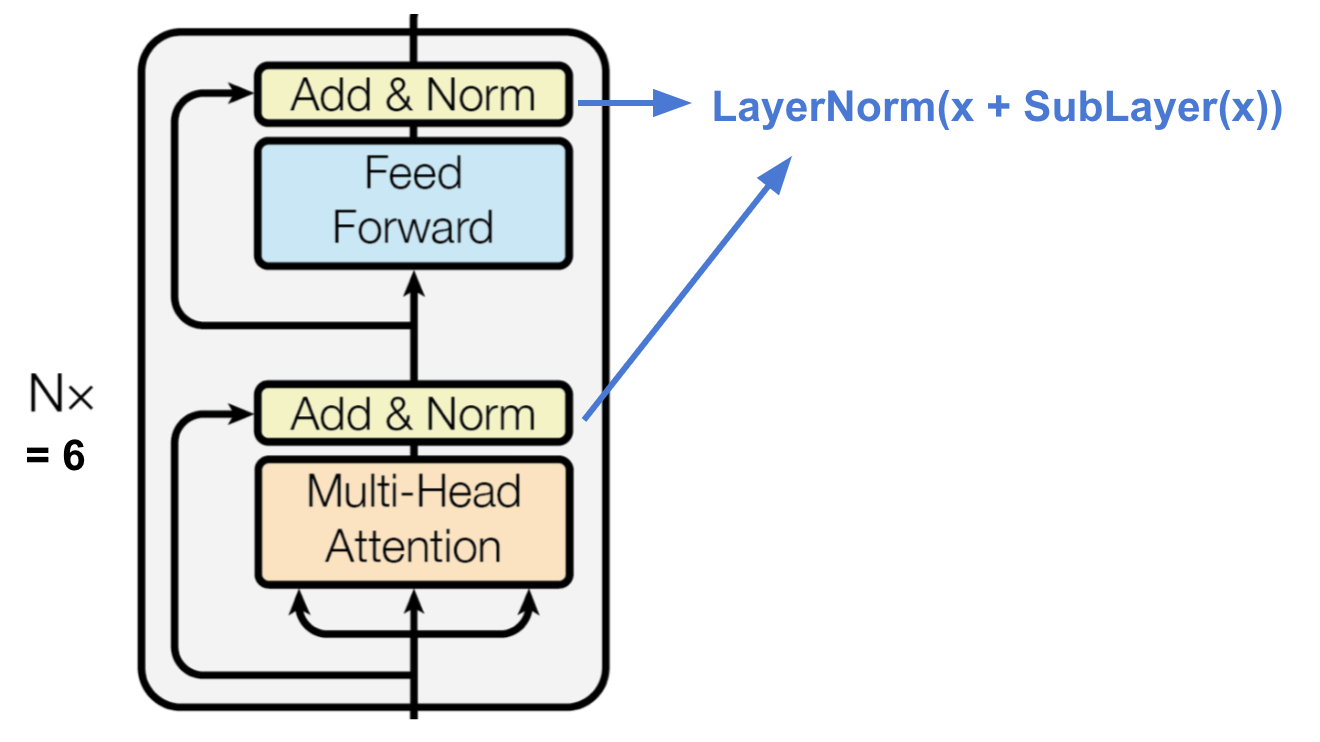
FIGURE 8.5: Single layer of the Encoder of a Transformer with two distinct sub-layers each with residual connections and a LayerNorm. Original image: (Vaswani et al. 2017), Additions and cropping: (Weng 2018)

The encoder is composed of a stack of N = 6 identical layers. Each of these layers has two sub-layers: A multi-head self-attention mechanism and a position-wise fully connected feed-forward network. The sub-layers have a residual connection around the main components which is followed by a layer normalization. The output of each sub-layer is \(\text{LayerNorm}(x + \text{Sublayer}(x))\) where \(\text{Sublayer}(x)\) is the output of the function of the sublayer itself. All sub-layers and the embedding layer before the encoder/decoder produce outputs of \(dim = d_{model} = 512\) to allow these residual connections to work. The position-wise feed-forward network used in the sublayer is applied to each position separately and identically. This network consists of two linear transformations with a ReLU activation function in between:

\[ FFN(x) = max(0, xW_1 + b_1)W_2 + b_2 \]

The decoder is, as seen in Figure 8.6, composed of a stack of \(N = 6\) identical layers.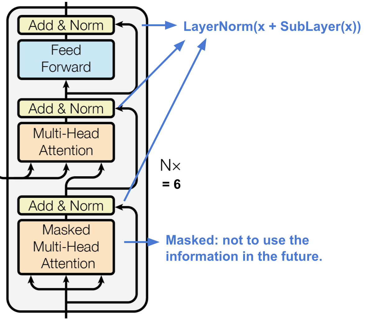

FIGURE 8.6: Decoder of a Transformer, Original image: (Vaswani et al. 2017), Additions and cropping: (Weng 2018)

It inserts, in addition to the two already known sub-layers from the encoder, a third sub-layer which also performs multi-head attention. This third sub-layer uses the encoder output as two of its three input values, which will be described in the next part of the chapter, for the multi-head attention. This sub-layer is in its function very close to the before seen attention mechanisms between encoders and decoders. It uses, same as the encoder, residual connections around each of the sub-layers. The decoder also uses a modified, masked self-attention sub-layer ``to prevent positions from attending to subsequent positions’’ Vaswani et al. (2017). This, coupled with the fact that the output embeddings are shifted by one position to the right ensures that the predictions for position \(i\) only depend on previous known outputs.

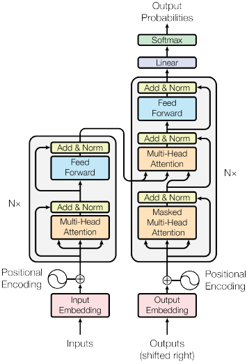
FIGURE 8.7: The Transformer-model architecture, Image Source: Fig. 1 in (Vaswani et al. 2017)

As seen in 8.7, the Transformer uses positional encodings added to the embeddings so the model can make use of the order of the sequence. Vaswani et al. (2017) use the sine and cosine function of different frequencies:

\[ PE_{(pos,2i)} = \sin(pos/10000^{2i/d_{model}}) \] \[ PE_{(pos,2i+1)} = \cos(pos/10000^{2i/d_{model}}) \] For further reasoning why these functions were chosen see Vaswani et al. (2017).

8.2.1.1 The self-attention mechanism(s)

Vaswani et al. (2017) describe attention functions as “mapping a query and a set of key-value pairs to an output, where the query, keys, values, and output are all vectors. The output is computed as a weighted sum of the values, where the weight assigned to each value is computed by a compatibility function of the query with the corresponding key”. The Query and the Key-Value pairs are used in the newly proposed attention mechanism that is used in Transformers. These inputs for the attention mechanisms are obtained through multiplication of the general input to the encoder/decoder with different weight matrices as can be seen in figure 8.8.

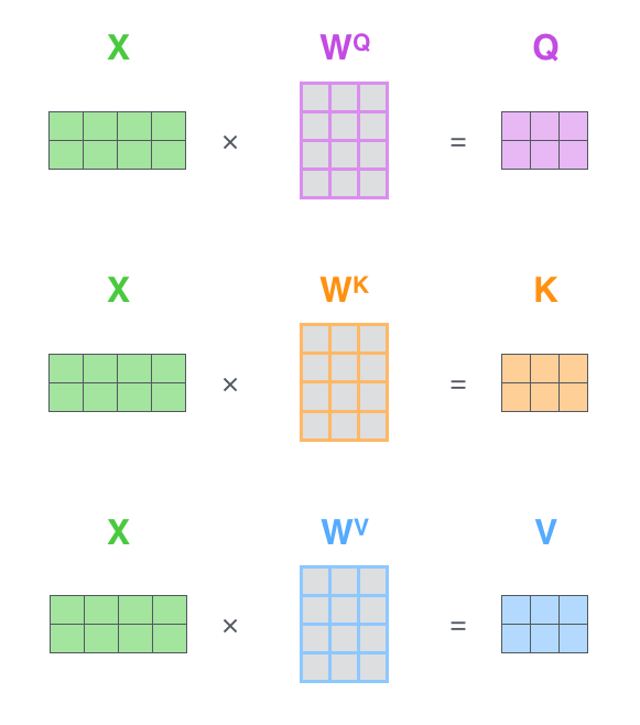
FIGURE 8.8: Input transformation used in a Transformer, \(Q = \text{Query}\), \(K = \text{Key}\), \(V = \text{Value}\). Image Source: (Alammar 2018)

These different transformations of the input are what enables the input to attend to itself. This in turn allows the model to learn about context. E.g. bank can mean very different things depending on the context which can be recognized by the self-attention mechanisms.

As seen in Figures 8.5, 8.6 and 8.7, the Transformer uses an attention mechanism called ``Multi-Head Attention’’.

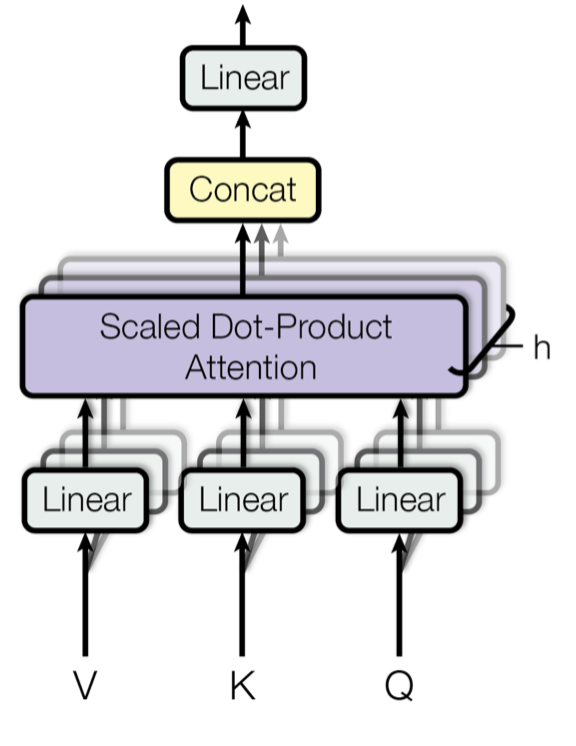
FIGURE 8.9: Multi-Head Attention, Image Source: Fig. 2 in (Vaswani et al. 2017)

The multi-head attention projects the queries, keys and values \(h\) times instead of performing a single attention on \(d_{model}\)-dim. queries and key-value pairs. The projections are learned, linear and project to \(d_k\), \(d_k\) and \(d_v\) dimensions. Next the new scaled dot-product attention is used on each of these to yield a \(d_v\)-dim. output. These values are then concatenated and projected to yield the final values as can be seen in 8.9. This multi-dimensionality allows the attention mechanism to jointly attend to different information from different representation at different positions. The multi-head attention can be written as:

\[ \text{MultiHead}(Q,K,V) = \text{Concat}(\text{head}_1,\dots, \text{head}_h)W^O \]

\[ \text{where } \text{head}_i = \text{Attention}(QW_i^Q, KW_i^K, VW_i^V) \] and projections are the parameter matrices \(W_i^Q\in \mathbb{R}^{d_{model}\times d_k}, W_i^K\in \mathbb{R}^{d_{model}\times d_k}, W_i^V\in \mathbb{R}^{d_{model}\times d_v}\text{ and } W^O\in \mathbb{R}^{hd_{v}\times d_{model}}\). Vaswani et al. (2017) use \(h = 8\) and \(d_k = d_v = d_{model}/h = 64\). This reduced dimensionality leads to a reduction in computational cost that is similar to that of a single scaled-dot-product attention head with the full initial dimensionality of \(512\).

The scaled dot-product attention is, as the name suggests, just a scaled version of the dot-product attention seen previously in this chapter.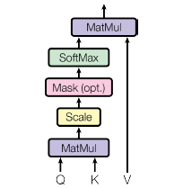

FIGURE 8.10: Scaled Dot-Product Attention, Image Source: Fig. 2 in (Vaswani et al. 2017)

The optional Mask-function seen in Fig. 8.10 is only used in the masked-multi-head attention of the decoder. The querys and keys are of dim. \(d_k\) and the values are of dim. \(d_v\). The attention is for practical reasons computed for a set of queries, Q. The keys and values are thus also used in matrix format, K and V. The matrix of outputs is then computed as:

\[ \text{Attention}(Q,K,V) = \text{softmax}(\frac{QK^\top}{\sqrt{d_k}})V \] where \(\text{Attention}(Q,K,V)\) corresponds to an non-projected head of multi-head attention. These attention mechanisms allow Transformers to learn different and distant dependencies in language and are thus a good candidate for transfer learning.

8.2.1.2 Complexity for different attention models

The architecture of a Transformer allows for parallel encoding of every part of the input at the same time. This also enables the modelling of long-range dependencies regardless of the distance. The Transformer architecture, as a minimum, only needs a constant number of sequential operations regardless of input length \(n\) due to extensive parallelization as can be seen in Table 8.2. A RNN based model in comparison needs a linearly scaling number of sequential operations due to its architecture. The Maximum Path Length between long-range dependencies for a transformer is \(O(1)\) while the RNN again has \(O(n)\) due to its sequential input reading.

The fast modelling of long-range dependencies and the multiple attention heads which learn different dependencies makes Transformers a favourable choice for Transfer Learning. The transfer learning models that were developed from the Transformer architecture enabled models which were trained on more data to gain a deeper understanding about language and are state-of-the-art today (June, 2020).

They are also a popular research topic as they are quadratically scaling, with regard to input length, complexity per layer inhibits their use for very long sequences and makes them time consuming to train. This quadratic complexity comes from the self-attention mechanism \(\text{Attention}(Q,K,V) = \text{softmax}(\frac{QK^\top}{\sqrt{d_k}})V\). The used softmax needs to calculate the attention score between the currently processed input \(x_i\) and every other input \(x_j\) for each \(j \in {1, \dots ,n}\) and \(i \in {1, \dots ,n}\). This limits the length of the context that Transformers can process and increases the time they need for training in practical uses. The computational costs are especially severe in very long tasks.

In the last few years new variations of the vanilla transformer, as described previously in the chapter, were published which lower the computational cost (e.g. Shen et al. (2018) and Choromanski et al. (2020)). Some of these variations of the Transformer architecture managed to decrease the complexity from quadratic to \(O(N\sqrt{N})\) (Child et al. (2019)), \(O(N\log N)\) (Kitaev, Kaiser, and Levskaya (2020)) or \(O(n)\) (Wang et al. (2020)) as seen in Table 8.2.

Layer-type	Complexity per Layer	Sequential Operations
Recurrent	\(O(n \cdot d^2)\)	\(O(n)\)
Convolutional	\(O(k \cdot n \cdot d^2)\)	\(O(1)\)
Transfomer	\(O(n^2 \cdot d)\)	\(O(1)\)
Sparse Transfomer	\(O(n\sqrt{n})\)	\(O(1)\)
Reformer	\(O(n \log (n))\)	\(O(\log (n))\)
Linformer	\(O(n)\)	\(O(1)\)
Linear Transformer	\(O(n)\)	\(O(1)\)

Table 8.2 : (#tab:complexity-operations) Complexity per layer and the number of sequential operations. Sparse Transformers are from Child et al. (2019), Reformer from Kitaev, Kaiser, and Levskaya (2020), Linformer from Wang et al. (2020) and Linear Transformers from Katharopoulos et al. (2020). \(n\) is the sequence length, \(k\) the kernel size, \(d\) the representation dimension and \(r\) the size of the neighbourhood in restricted self-attention. Source: Vaswani et al. (2017) (Table 1) and Wang et al. (2020) (Table 1)

8.2.2 Transformers as RNNs

A version from Katharopoulos et al. (2020) uses a linear attention mechanism for autoregressive tasks. The vanilla Transformer uses, as described above, the softmax to calculate the attention between values. This can also be seen as a similarity function. \(V_i' = \frac{\sum_{j=1}^N \text{sim}(Q_i, K_j)V_j}{\sum_{j=1}^N\text{sim}(Q_i, K_j)}\) is equal to the row-wise calculation of \(\text{Attention}(Q,K,V) = V' = \text{softmax}(\frac{QK^\top}{\sqrt{d_k}})V\) if \(\text{sim}(q,k)=\exp(\frac{q^\top k}{\sqrt{d_k}})\). While we can use the exponentiated dot-product to generate the vanilla scaled-dot-product attention, we can use any non-negative function, including kernels, as similarity function to generate a new attention mechanism Katharopoulos et al. (2020). Given the feature representation \(\phi(x)\) of such a kernel, the previous row-wise calculation can be rewritten as \(V_i' = \frac{\phi(Q_i)^\top \sum_{j=1}^N\phi(K_j)V_j^\top}{\phi(Q_i)^\top \sum_{j=1}^N\phi(K_j)}\). Or in vectorized form: \(\phi(Q)(\phi(K)^\top V)\) where the feature map \(\phi(\cdot)\) is applied row-wise to the matrices. This new formulation shows that the computation with a feature map allows for linear time and memory scaling \(O(n)\) because \(\sum_{j=1}^N\phi(K_j)V_j^\top\) and \(\sum_{j=1}^N\phi(K_j)\) can be both computed once and reused for every row of the query (Katharopoulos et al. (2020)). No finite dimensional feature map of the exponential function exists, which makes a linearisation of the softmax attention impossible. This forces the use of a polynomial kernel which has been shown to work equally well with the exponential kernel Tsai et al. (2019). This results in a computational cost of \(O(ND^2M)\) which is favourable if \(N > D^2\). Katharopoulos et al. (2020) suggest \(\phi(x) = \text{elu}(x) + 1\) for \(N < D^2\).

For autoregressive tasks we want an attention mechanism that can’t look ahead of its position. Vaswani et al. (2017) introduced masked-self-attention for their decoder, which is adapted for linearised attention. The addition of masking changes the previous formulation to \(V_i' = \frac{\sum_{j=1}^i \text{sim}(Q_i, K_j)V_j}{\sum_{j=1}^i\text{sim}(Q_i, K_j)}\). With the linearisation through kernels we get \(V_i' = \frac{\phi(Q_i)^\top \sum_{j=1}^i\phi(K_j)V_j^\top}{\phi(Q_i)^\top \sum_{j=1}^i\phi(K_j)}\).

\(S_i = \sum_{j=1}^i\phi(K_j)V_j^\top\) and \(Z_i = \sum_{j=1}^i\phi(K_j)\) can be used to simplify the formula to:

\[ V_i' = \frac{\phi(Q_i)^\top Si}{\phi(Q_i)^\top Z_i} \]

where \(S_i\) and \(Z_i\) can be computed from \(S_{i-1}\) and \(Z_{i-1}\) which allows the linearised attention with masking to scale linearly with respect to the sequence length. The derivation of the numerator as cumulative sums allows for the computation in linear time and constant memory, which leads to computational complexity of \(O(NCM)\) and memory \(O(N \max{(C,d_k)})\) where \(C\) is the dimensionality of the feature map Katharopoulos et al. (2020).

Given the previous formalization of feature maps to replace the softmax we can rewrite the layers of a Transformers as a RNN. This RNN has two hidden states, the attention state \(s\) and the normalizer state \(z\) with subscripts denoting the timestep in recurrence. With \(s_0 = 0\) and \(z_0 = 0\) we can define \(s_i\) as \(s_i s_{i-1} + \phi(x_iW_K)(x_iW_V)^\top\) and \(z_i\) as \(z_i = z_{i-1} + \phi(x_iW_K)\) with \(x_i\) as the \(i\)-th input for the layer. The \(i\)-th output \(y_i\) can then be written as \(y_i = f_l(\frac{\phi(x_iW_Q)^\top s_i}{\phi(x_iW_Q)^\top z_i} + x_i)\) where \(f_l\) is the function given by the feed-forward network of a Transformer layer.

This shows that the Transformer layers can be rewritten into RNN layers, for all similarity functions that can be represented with \(\phi\) (Katharopoulos et al. (2020)), which are the first models that used attention for NLP tasks.

References

Alammar, Jay. 2018. “The Illustrated Transformer [Blog Post].” Http://Jalammar.github.io/. http://jalammar.github.io/illustrated-transformer/.

Bahdanau, Dzmitry, Kyunghyun Cho, and Yoshua Bengio. 2014. “Neural Machine Translation by Jointly Learning to Align and Translate.” arXiv Preprint arXiv:1409.0473.

Cheng, Jianpeng, Li Dong, and Mirella Lapata. 2016. “Long Short-Term Memory-Networks for Machine Reading.” arXiv Preprint arXiv:1601.06733.

Child, Rewon, Scott Gray, Alec Radford, and Ilya Sutskever. 2019. “Generating Long Sequences with Sparse Transformers.”

Choromanski, Krzysztof, Valerii Likhosherstov, David Dohan, Xingyou Song, Jared Davis, Tamas Sarlos, David Belanger, Lucy Colwell, and Adrian Weller. 2020. “Masked Language Modeling for Proteins via Linearly Scalable Long-Context Transformers.”

Gehring, Jonas, Michael Auli, David Grangier, Denis Yarats, and Yann N. Dauphin. 2017. “Convolutional Sequence to Sequence Learning.”

Graves, Alex, Greg Wayne, and Ivo Danihelka. 2014. “Neural Turing Machines.” CoRR abs/1410.5401. http://arxiv.org/abs/1410.5401.

Gregor, Karol, Ivo Danihelka, Alex Graves, Danilo Jimenez Rezende, and Daan Wierstra. 2015. “Draw: A Recurrent Neural Network for Image Generation.” arXiv Preprint arXiv:1502.04623.

Kalchbrenner, Nal, Lasse Espeholt, Karen Simonyan, Aaron van den Oord, Alex Graves, and Koray Kavukcuoglu. 2016a. “Neural Machine Translation in Linear Time.”

Katharopoulos, Angelos, Apoorv Vyas, Nikolaos Pappas, and François Fleuret. 2020. “Transformers Are Rnns: Fast Autoregressive Transformers with Linear Attention.”

Kitaev, Nikita, Łukasz Kaiser, and Anselm Levskaya. 2020. “Reformer: The Efficient Transformer.”

Luong, Minh-Thang, Hieu Pham, and Christopher D Manning. 2015. “Effective Approaches to Attention-Based Neural Machine Translation.” arXiv Preprint arXiv:1508.04025.

Shen, Zhuoran, Mingyuan Zhang, Haiyu Zhao, Shuai Yi, and Hongsheng Li. 2018. “Efficient Attention: Attention with Linear Complexities.”

Sutskever, Ilya, Oriol Vinyals, and Quoc V Le. 2014. “Sequence to Sequence Learning with Neural Networks.” In Advances in Neural Information Processing Systems, 3104–12.

Tsai, Yao-Hung Hubert, Shaojie Bai, Makoto Yamada, Louis-Philippe Morency, and Ruslan Salakhutdinov. 2019. “Transformer Dissection: A Unified Understanding of Transformer’s Attention via the Lens of Kernel.”

Vaswani, Ashish, Noam Shazeer, Niki Parmar, Jakob Uszkoreit, Llion Jones, Aidan N Gomez, Łukasz Kaiser, and Illia Polosukhin. 2017. “Attention Is All You Need.” In Advances in Neural Information Processing Systems, 5998–6008.

Wang, Sinong, Belinda Z. Li, Madian Khabsa, Han Fang, and Hao Ma. 2020. “Linformer: Self-Attention with Linear Complexity.”

Weng, Lilian. 2018. “Attention? Attention!” Lilianweng.github.io/Lil-Log. http://lilianweng.github.io/lil-log/2018/06/24/attention-attention.html.

Xu, Kelvin, Jimmy Ba, Ryan Kiros, Kyunghyun Cho, Aaron Courville, Ruslan Salakhudinov, Rich Zemel, and Yoshua Bengio. 2015. “Show, Attend and Tell: Neural Image Caption Generation with Visual Attention.” In International Conference on Machine Learning, 2048–57.