Visualization of Objective Functions
objective_functions.RmdThis vignette covers the basic usage of objective functions in
vistool, including predefined objectives and how to define
custom objectives.
Predefined Objectives
The package provides a dictionary of objective functions:
as.data.table(dict_objective)
#> Key: <key>
#> key label xdim lower upper
#> <char> <char> <int> <list> <list>
#> 1: TF_Gfunction Gfunction NA NA NA
#> 2: TF_GoldsteinPrice GoldsteinPrice 2 0,0 1,1
#> 3: TF_GoldsteinPriceLog GoldsteinPriceLog 2 0,0 1,1
#> 4: TF_OTL_Circuit OTL_Circuit 6 NA NA
#> 5: TF_RoosArnold RoosArnold NA NA NA
#> 6: TF_ackley ackley 2 0,0 1,1
#> 7: TF_banana banana 2 0,0 1,1
#> 8: TF_beale beale 2 0,0 1,1
#> 9: TF_borehole borehole 2 0,0 1.5,1.0
#> 10: TF_branin branin 2 -2,-2 3,3
#> 11: TF_currin1991 currin1991 2 0,0 1,1
#> 12: TF_easom easom 2 0,0 1,1
#> 13: TF_franke franke 2 -0.5,-0.5 1,1
#> 14: TF_gaussian1 gaussian1 NA NA NA
#> 15: TF_griewank griewank NA NA NA
#> 16: TF_hartmann hartmann 6 NA NA
#> 17: TF_hump hump 2 0,0 1,1
#> 18: TF_levy levy NA NA NA
#> 19: TF_linkletter_nosignal linkletter_nosignal NA NA NA
#> 20: TF_michalewicz michalewicz NA NA NA
#> 21: TF_piston piston 7 NA NA
#> 22: TF_powsin powsin NA NA NA
#> 23: TF_quad_peaks quad_peaks 2 0,0 1,1
#> 24: TF_quad_peaks_slant quad_peaks_slant 2 0,0 1,1
#> 25: TF_rastrigin rastrigin NA NA NA
#> 26: TF_robotarm robotarm 8 NA NA
#> 27: TF_sinumoid sinumoid 2 0,0 1,1
#> 28: TF_sqrtsin sqrtsin NA NA NA
#> 29: TF_waterfall waterfall 2 0,0 1,1
#> 30: TF_wingweight wingweight 10 NA NA
#> 31: TF_zhou1998 zhou1998 2 0,0 1,1
#> key label xdim lower upperTo retrieve an objective function:
obj_branin = obj("TF_branin")You can evaluate the objective, gradient, and Hessian at a point:
x = c(0.9, 1)
obj_branin$eval(x)
#> [1] 178.3166
obj_branin$grad(x)
#> [1] -354.3258 395.8377
obj_branin$hess(x)
#> [,1] [,2]
#> [1,] -1989.5197 -284.2171
#> [2,] -284.2171 2162.1162Visualizing Objectives
Use as_visualizer() to create a visualizer for an
objective. For 1D and 2D objectives, the appropriate visualizer is
selected automatically.
viz = as_visualizer(obj_branin)
viz$plot()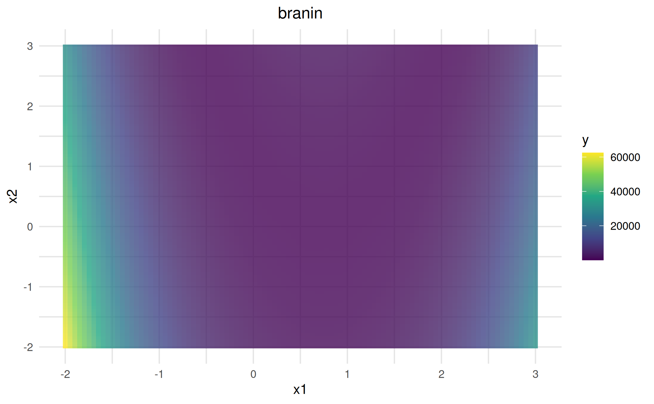
For interactive surface visualization (2D objectives):
viz_surface = as_visualizer(obj_branin, type = "surface")
viz_surface$plot()Transformed to a contour plot:
viz_surface$plot(flatten = TRUE)Custom Objectives
You can define your own objective function. Let’s define a loss for a
linear model on the iris data with target Sepal.Width and
feature Petal.Width. First, an Objective
requires a function for evaluation:
# Define the linear model loss function as SSE:
l2norm = function(x) sqrt(sum(crossprod(x)))
mylm = function(x, Xmat, y) {
l2norm(y - Xmat %*% x)
}To fix the loss for the data, the Objective$new() call
allows to pass custom arguments that are stored and reused in every call
to $eval() to evaluate fun. So, calling
$eval(x) internally calls fun(x, ...). These
arguments must be specified just once:
# Use the iris dataset with response `Sepal.Width` and feature `Petal.Width`:
Xmat = model.matrix(~Petal.Width, data = iris)
y = iris$Sepal.Width
# Create a new object:
obj_lm = Objective$new(id = "iris LM", fun = mylm, xdim = 2, Xmat = Xmat, y = y, minimize = TRUE)
obj_lm$evalStore(c(1, 2))
obj_lm$evalStore(c(2, 3))
obj_lm$evalStore(coef(lm(Sepal.Width ~ Petal.Width, data = iris)))
obj_lm$archive
#> x fval grad gnorm
#> <list> <num> <list> <num>
#> 1: 1,2 21.553654 2.375467,11.722838 1.196109e+01
#> 2: 2,3 43.410022 8.779078,16.929270 1.907020e+01
#> 3: 3.3084256,-0.2093598 4.951004 4.832272e-07,2.664535e-07 5.518206e-07Visualize the custom objective:
viz_lm = as_visualizer(obj_lm, x1_limits = c(-0.5, 5), x2_limits = c(-3.2, 2.8))
viz_lm$plot()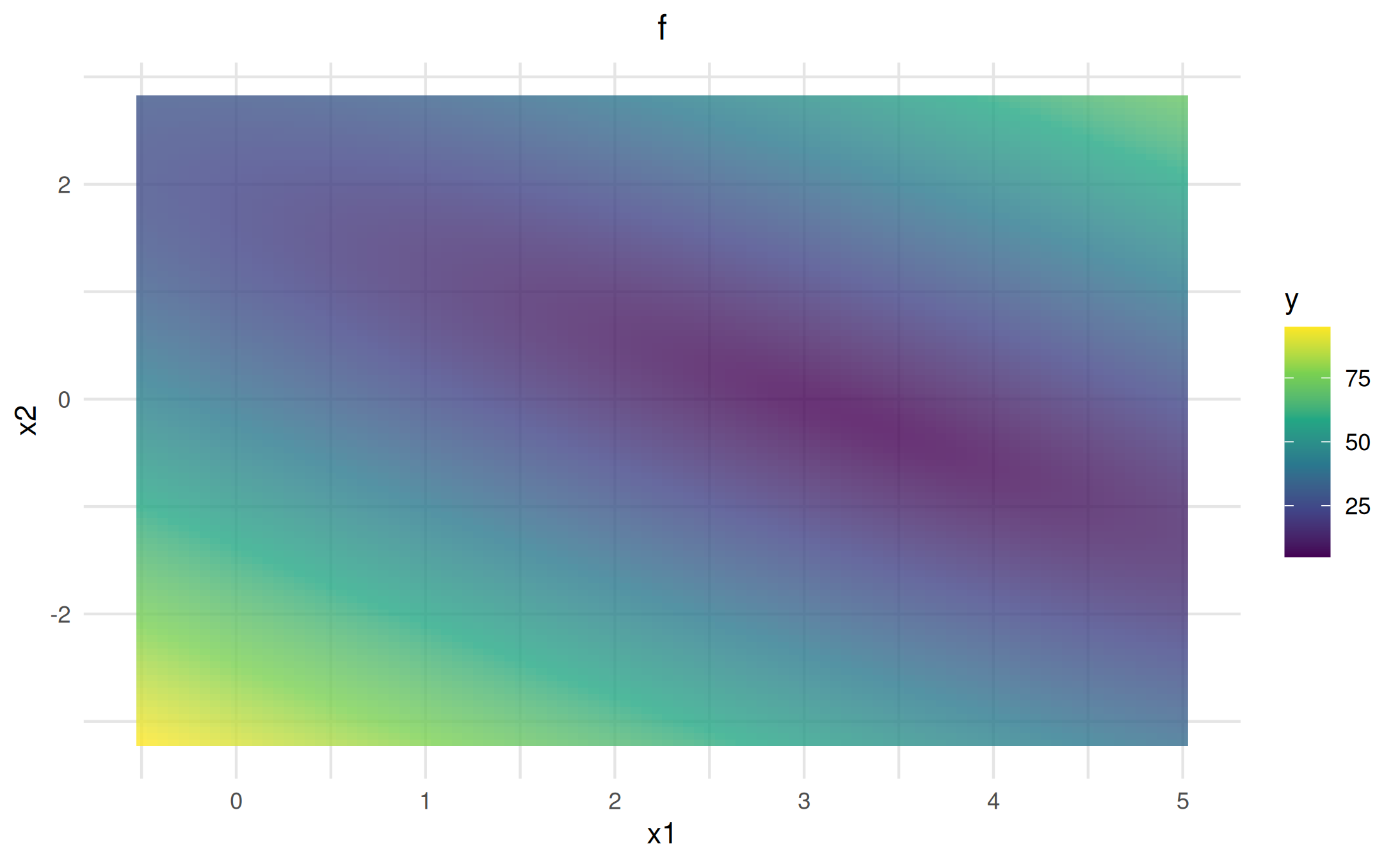
You can also add custom points directly to the visualizer using
$add_points(), which supports many customization options
(see below). For adding actual optimization traces, see the Optimization & Traces
vignette.
archive_data = data.frame(
x = sapply(obj_lm$archive$x, function(x) x[1]),
y = sapply(obj_lm$archive$x, function(x) x[2])
)
viz_lm$add_points(archive_data, color = "orange", size = 3, shape = 17, alpha = 0.8, ordered = TRUE)$plot()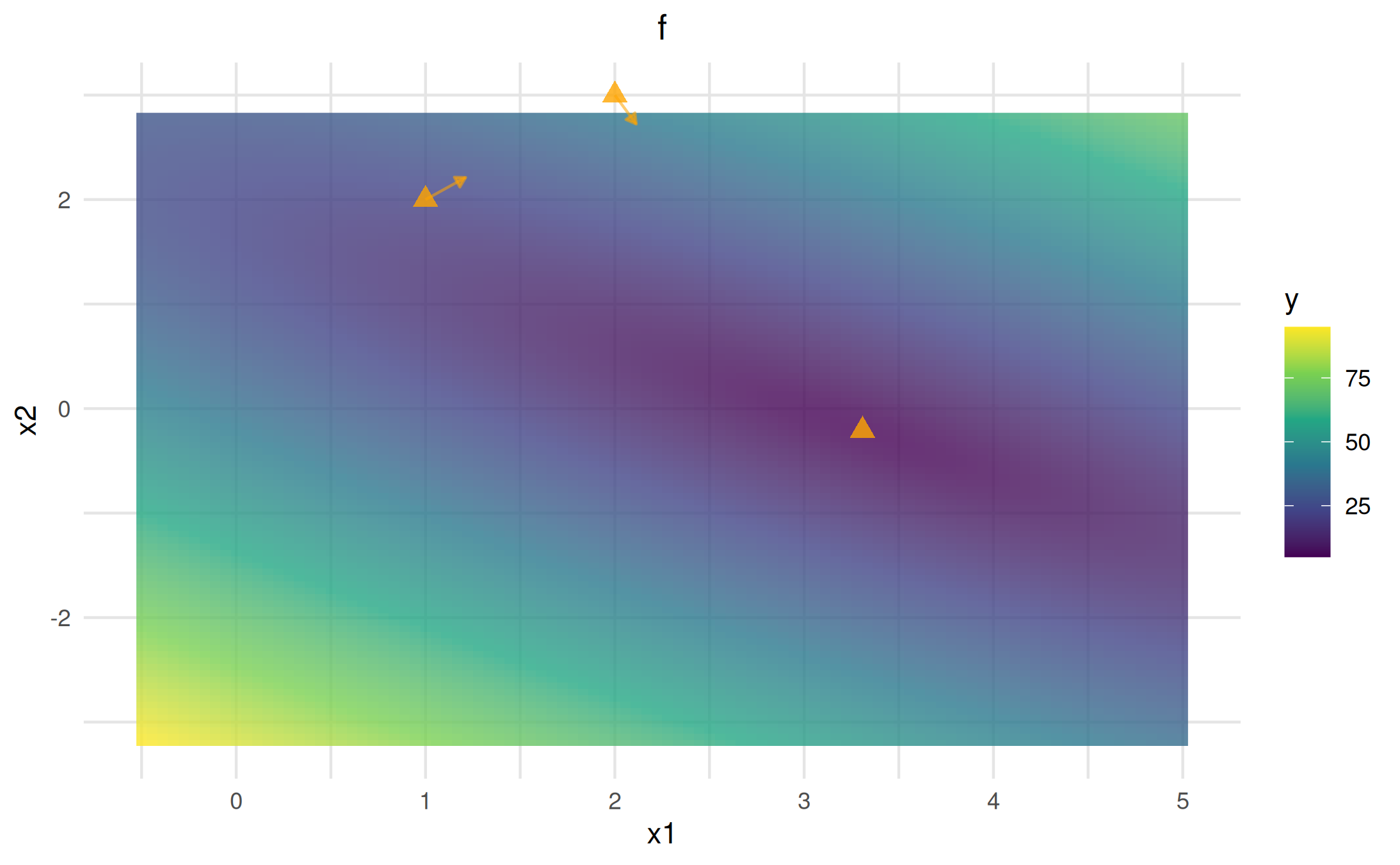
# Add a labeled point to the surface (plotly) visualizer
viz_lm_surface = as_visualizer(obj_lm, x1_limits = c(-0.5, 5), x2_limits = c(-3.2, 2.8), type = "surface")
viz_lm_surface$add_points(base::data.frame(x = 2, y = 0), color = "orange", size = 8, alpha = 0.9, annotations = "The z values are inferred!")$plot()Customization options include: points (as
data.frame/matrix/list), color, size,
shape, alpha, annotations,
ordered, and more. See the documentation for all
arguments.