Optimization & traces
optimization_traces.RmdThis vignette covers the available optimizers, step size control, and how to visualize optimization traces.
Optimizers
The optimizer class defines the optimization strategy and is initialized by taking an objective function, start value, and learning rate. Available optimizers are:
- Gradient descent with
OptimizerGD - Momentum with
OptimizerMomentum - Nesterov’s momentum with
OptimizerNAG
Creating an optimizer is done by (let’s use an x value that works well):
obj = obj("TF_GoldsteinPriceLog")
opt = OptimizerGD$new(obj, x_start = c(0.22, 0.77), lr = 0.01)
With these values set, run $optimize() with the number
of steps:
opt$optimize(10L)
#> TF_GoldsteinPriceLog: Batch 1 step 1: f(x) = 0.9158, x = c(0.219, 0.7186)
#> TF_GoldsteinPriceLog: Batch 1 step 2: f(x) = 0.4217, x = c(0.211, 0.6549)
#> TF_GoldsteinPriceLog: Batch 1 step 3: f(x) = -0.6741, x = c(0.1844, 0.5649)
#> TF_GoldsteinPriceLog: Batch 1 step 4: f(x) = -0.9819, x = c(0.2182, 0.5224)
#> TF_GoldsteinPriceLog: Batch 1 step 5: f(x) = -0.9876, x = c(0.2992, 0.5105)
#> TF_GoldsteinPriceLog: Batch 1 step 6: f(x) = -1.1018, x = c(0.2625, 0.3598)
#> TF_GoldsteinPriceLog: Batch 1 step 7: f(x) = -2.168, x = c(0.3405, 0.4107)
#> TF_GoldsteinPriceLog: Batch 1 step 8: f(x) = -2.1246, x = c(0.3448, 0.3898)
#> TF_GoldsteinPriceLog: Batch 1 step 9: f(x) = -1.3408, x = c(0.4093, 0.4614)
#> TF_GoldsteinPriceLog: Batch 1 step 10: f(x) = -2.1225, x = c(0.3729, 0.3911)
Calling $optimize() also writes into the archive of the
optimizer and also calls $eval_store() of the objective.
Therefore, $optimize() writes into two archives:
opt$archive
#>                   x_out                x_in                    update
#>                  <list>              <list>                    <list>
#>  1: 0.2189909,0.7185977           0.22,0.77 -0.001009067,-0.051402328
#>  2: 0.2109802,0.6548741 0.2189909,0.7185977   -0.00801070,-0.06372357
#>  3: 0.1844147,0.5648984 0.2109802,0.6548741   -0.02656552,-0.08997572
#>  4: 0.2182254,0.5223500 0.1844147,0.5648984    0.03381065,-0.04254834
#>  5: 0.2992118,0.5105193 0.2182254,0.5223500    0.08098642,-0.01183078
#>  6: 0.2625368,0.3597982 0.2992118,0.5105193   -0.03667496,-0.15072102
#>  7: 0.3405450,0.4106795 0.2625368,0.3597982     0.07800819,0.05088128
#>  8: 0.3448264,0.3897982 0.3405450,0.4106795  0.004281407,-0.020881313
#>  9: 0.4092595,0.4613701 0.3448264,0.3897982     0.06443313,0.07157191
#> 10: 0.3728515,0.3910876 0.4092595,0.4613701   -0.03640808,-0.07028256
#>       fval_out    fval_in    lr step_size         objective_id momentum  step
#>          <num>      <num> <num>     <num>               <char>    <num> <int>
#>  1:  0.9157526  1.2102644  0.01         1 TF_GoldsteinPriceLog        0     1
#>  2:  0.4217145  0.9157526  0.01         1 TF_GoldsteinPriceLog        0     2
#>  3: -0.6741307  0.4217145  0.01         1 TF_GoldsteinPriceLog        0     3
#>  4: -0.9818620 -0.6741307  0.01         1 TF_GoldsteinPriceLog        0     4
#>  5: -0.9876309 -0.9818620  0.01         1 TF_GoldsteinPriceLog        0     5
#>  6: -1.1017546 -0.9876309  0.01         1 TF_GoldsteinPriceLog        0     6
#>  7: -2.1680122 -1.1017546  0.01         1 TF_GoldsteinPriceLog        0     7
#>  8: -2.1245834 -2.1680122  0.01         1 TF_GoldsteinPriceLog        0     8
#>  9: -1.3408109 -2.1245834  0.01         1 TF_GoldsteinPriceLog        0     9
#> 10: -2.1225452 -1.3408109  0.01         1 TF_GoldsteinPriceLog        0    10
#>     batch
#>     <num>
#>  1:     1
#>  2:     1
#>  3:     1
#>  4:     1
#>  5:     1
#>  6:     1
#>  7:     1
#>  8:     1
#>  9:     1
#> 10:     1
opt$objective$archive
#>                       x       fval                  grad     gnorm
#>                  <list>      <num>                <list>     <num>
#>  1:           0.22,0.77  1.2102644   0.1009067,5.1402328  5.141223
#>  2: 0.2189909,0.7185977  0.9157526     0.801070,6.372357  6.422511
#>  3: 0.2109802,0.6548741  0.4217145     2.656552,8.997572  9.381555
#>  4: 0.1844147,0.5648984 -0.6741307   -3.381065, 4.254834  5.434631
#>  5: 0.2182254,0.5223500 -0.9818620   -8.098642, 1.183078  8.184600
#>  6: 0.2992118,0.5105193 -0.9876309    3.667496,15.072102 15.511892
#>  7: 0.2625368,0.3597982 -1.1017546   -7.800819,-5.088128  9.313529
#>  8: 0.3405450,0.4106795 -2.1680122 -0.4281407, 2.0881313  2.131571
#>  9: 0.3448264,0.3897982 -2.1245834   -6.443313,-7.157191  9.630247
#> 10: 0.4092595,0.4613701 -1.3408109     3.640808,7.028256  7.915293
Visualize optimization traces
A layer of the Visualizer class is
$add_optimization_trace() that gets the optimizer as
argument and adds the optimization trace to the plot:
vis = as_visualizer(obj, type = "surface")
vis$add_optimization_trace(opt, name = "GD")
vis$plot()
Step size control
$optimize() accepts a second argument
step_size_control to scale the parameter update. For GD
with
,
the update
is multiplied by the return value of step_size_control().
There are a few pre-implemented control functions like line search or
various decaying methods:
-
step_size_control_line_search(lower, upper): Conduct a line search for in . -
step_size_control_decay_time(decay): Lower the updates by . -
step_size_control_decay_exp(decay): Lower the updates by . -
step_size_control_decay_linear(iter_zero): Lower the updates untiliter_zerois reached. Updates withiter > iter_zeroare 0. -
step_size_control_decay_steps(drop_rate, every_iter): Lower the updatesevery_iterbydrop_rate.
Note that these functions return a function that contains a function with the required signature:
step_size_control_decay_time()
#> function (x, u, obj, opt)
#> {
#>     assert_step_size_control(x, u, obj, opt)
#>     epoch = nrow(obj$archive)
#>     return(1/(1 + decay * epoch))
#> }
#> <bytecode: 0x55b2bb359dc8>
#> <environment: 0x55b2bb354a50>
Let’s define multiple gradient descent optimizers and optimize 10 steps with a step size control:
x0 = c(0.22, 0.77)
lr = 0.01

oo1 = OptimizerGD$new(obj, x_start = x0, lr = lr, id = "GD without LR Control", print_trace = FALSE)
oo2 = OptimizerGD$new(obj, x_start = x0, lr = lr, id = "GD with Line Search", print_trace = FALSE)
oo3 = OptimizerGD$new(obj, x_start = x0, lr = lr, id = "GD with Time Decay", print_trace = FALSE)
oo4 = OptimizerGD$new(obj, x_start = x0, lr = lr, id = "GD with Exp Decay", print_trace = FALSE)
oo5 = OptimizerGD$new(obj, x_start = x0, lr = lr, id = "GD with Linear Decay", print_trace = FALSE)
oo6 = OptimizerGD$new(obj, x_start = x0, lr = lr, id = "GD with Step Decay", print_trace = FALSE)

oo1$optimize(steps = 10)
oo2$optimize(steps = 10, step_size_control_line_search())
oo3$optimize(steps = 10, step_size_control_decay_time())
oo4$optimize(steps = 10, step_size_control_decay_exp())
oo5$optimize(steps = 10, step_size_control_decay_linear())
oo6$optimize(steps = 10, step_size_control_decay_steps())
For now we don’t know how well it worked. Let’s collect all archives
with merge_optim_archives() and visualize the step sizes
and function values with patchwork magic:
arx = merge_optim_archives(oo1, oo2, oo3, oo4, oo5, oo6)

library(ggplot2)
library(patchwork)
gg1 = ggplot(arx, aes(x = iteration, y = step_size, color = optim_id))
gg2 = ggplot(arx, aes(x = iteration, y = fval_out, color = optim_id))

(gg1 + ggtitle("Step sizes") |
  gg1 + ylim(0, 1) + ggtitle("Step sizes (zoomed)") |
  gg2 + ggtitle("Objective")) +
  plot_layout(guides = "collect") &
  geom_line() &
  theme_minimal() &
  theme(legend.position = "bottom") &
  ggsci::scale_color_simpsons()
#> Warning: Removed 2 rows containing missing values or values outside the scale range
#> (`geom_line()`).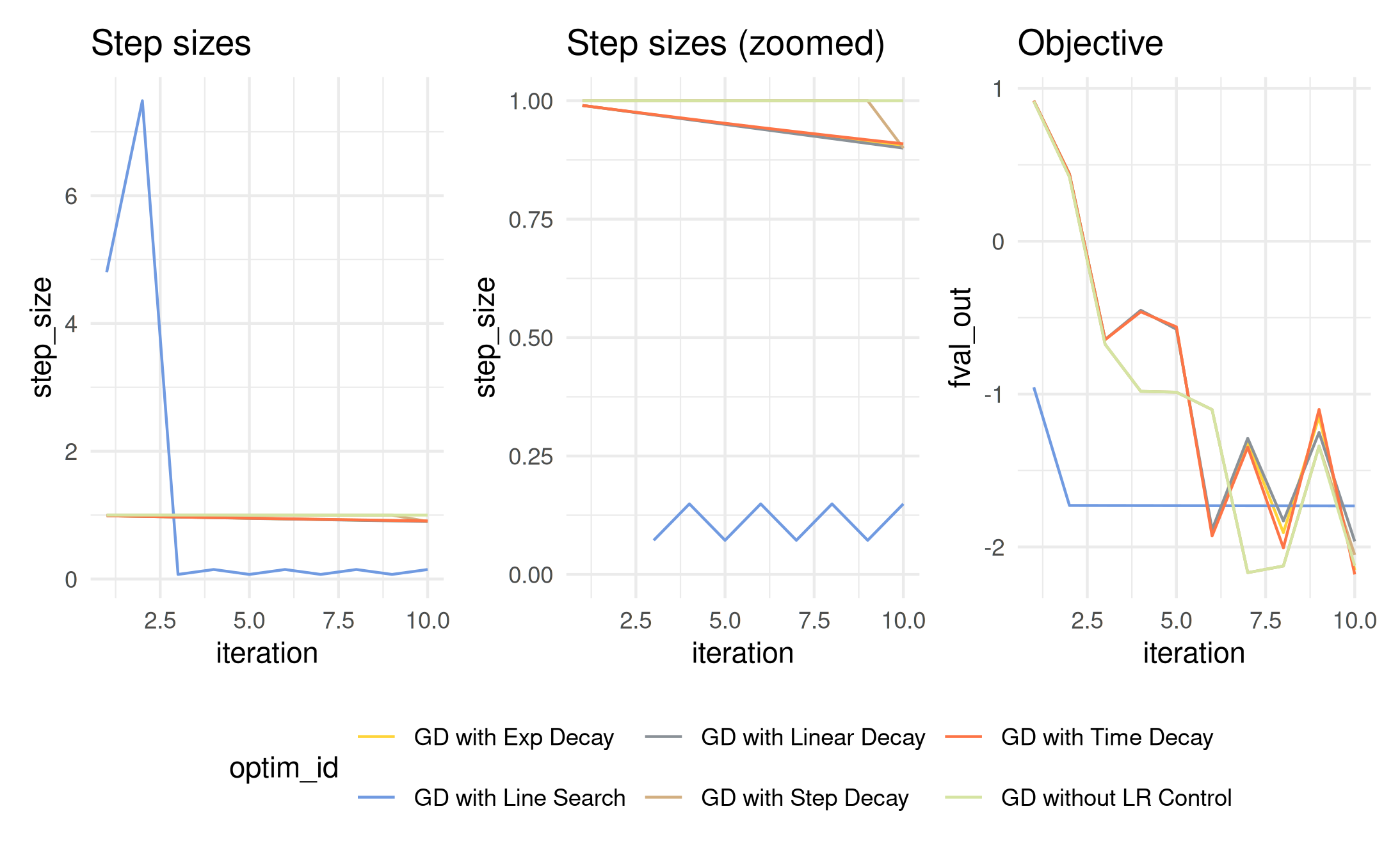
Visualizing the traces is done as before by adding optimization trace layer. We can do this for all optimizers to add multiple traces to the plot:
vis = as_visualizer(obj, type = "surface")

vis$add_optimization_trace(oo1)
vis$add_optimization_trace(oo2)
vis$add_optimization_trace(oo3)
vis$add_optimization_trace(oo4)
vis$add_optimization_trace(oo5)
vis$add_optimization_trace(oo6)

vis$plot()
Practically, it should be no issue to also combine multiple control
functions. The important thing is to keep the signature of the function
by allowing the function to get the arguments x (current
value), u (current update), obj
(Objective object), and opt
(Optimizer object):
myStepSizeControl = function(x, u, obj, opt) {
  sc1 = step_size_control_line_search(0, 10)
  sc2 = step_size_control_decay_time(0.1)
  return(sc1(x, u, obj, opt) * sc2(x, u, obj, opt))
}

my_oo = OptimizerGD$new(obj, x_start = x0, lr = lr, id = "GD without LR Control", print_trace = FALSE)
my_oo$optimize(100, myStepSizeControl)
tail(my_oo$archive)
#>        x_out      x_in                      update  fval_out   fval_in    lr
#>       <list>    <list>                      <list>     <num>     <num> <num>
#> 1: 0.50,0.25 0.50,0.25  4.440892e-10,-3.996803e-09 -3.129126 -3.129126  0.01
#> 2: 0.50,0.25 0.50,0.25 -2.664535e-09,-7.105427e-09 -3.129126 -3.129126  0.01
#> 3: 0.50,0.25 0.50,0.25 -3.552714e-09,-3.552714e-09 -3.129126 -3.129126  0.01
#> 4: 0.50,0.25 0.50,0.25   8.881784e-10,7.549517e-09 -3.129126 -3.129126  0.01
#> 5: 0.50,0.25 0.50,0.25  0.000000e+00,-1.021405e-08 -3.129126 -3.129126  0.01
#> 6: 0.50,0.25 0.50,0.25   8.881784e-10,0.000000e+00 -3.129126 -3.129126  0.01
#>      step_size         objective_id momentum  step batch
#>          <num>               <char>    <num> <int> <num>
#> 1: 0.015061886 TF_GoldsteinPriceLog        0    95     1
#> 2: 0.006942669 TF_GoldsteinPriceLog        0    96     1
#> 3: 0.010225887 TF_GoldsteinPriceLog        0    97     1
#> 4: 0.063947308 TF_GoldsteinPriceLog        0    98     1
#> 5: 0.006044013 TF_GoldsteinPriceLog        0    99     1
#> 6: 0.564836746 TF_GoldsteinPriceLog        0   100     1
Customization options
Let’s optimize a custom linear model objective (see the Objective functions vignette) using the three available optimizers.
# Define the linear model loss function as SSE:
l2norm = function(x) sqrt(sum(crossprod(x)))

mylm = function(x, Xmat, y) {
  l2norm(y - Xmat %*% x)
}
# Use the iris dataset with response `Sepal.Width` and feature `Petal.Width`:
Xmat = model.matrix(~Petal.Width, data = iris)
y = iris$Sepal.Width

# Create a new object:
obj_lm = Objective$new(id = "iris LM", fun = mylm, xdim = 2, Xmat = Xmat, y = y, minimize = TRUE)

oo1 = OptimizerGD$new(obj_lm, x_start = c(0, -0.05), lr = 0.001, print_trace = FALSE)
oo2 = OptimizerMomentum$new(obj_lm, x_start = c(3, 2), lr = 0.001, print_trace = FALSE)
oo3 = OptimizerNAG$new(obj_lm, x_start = c(1, -2), lr = 0.001, print_trace = FALSE)

oo1$optimize(steps = 100)
oo2$optimize(steps = 100)
oo3$optimize(steps = 100)
Optimization traces support many customization options (see the Customization guide):
vis = as_visualizer(obj_lm, x1_limits = c(-0.5, 5), x2_limits = c(-3.2, 2.8), type = "surface")
vis$add_optimization_trace(oo1, add_marker_at = round(seq(1, 100, len = 10L)))
vis$add_optimization_trace(oo2, line_color = "yellow", add_marker_at = c(1, 50, 90), marker_shape = c("square", "diamond", "cross"))
vis$add_optimization_trace(oo3, line_color = "red", line_width = 20, line_type = "dashed")
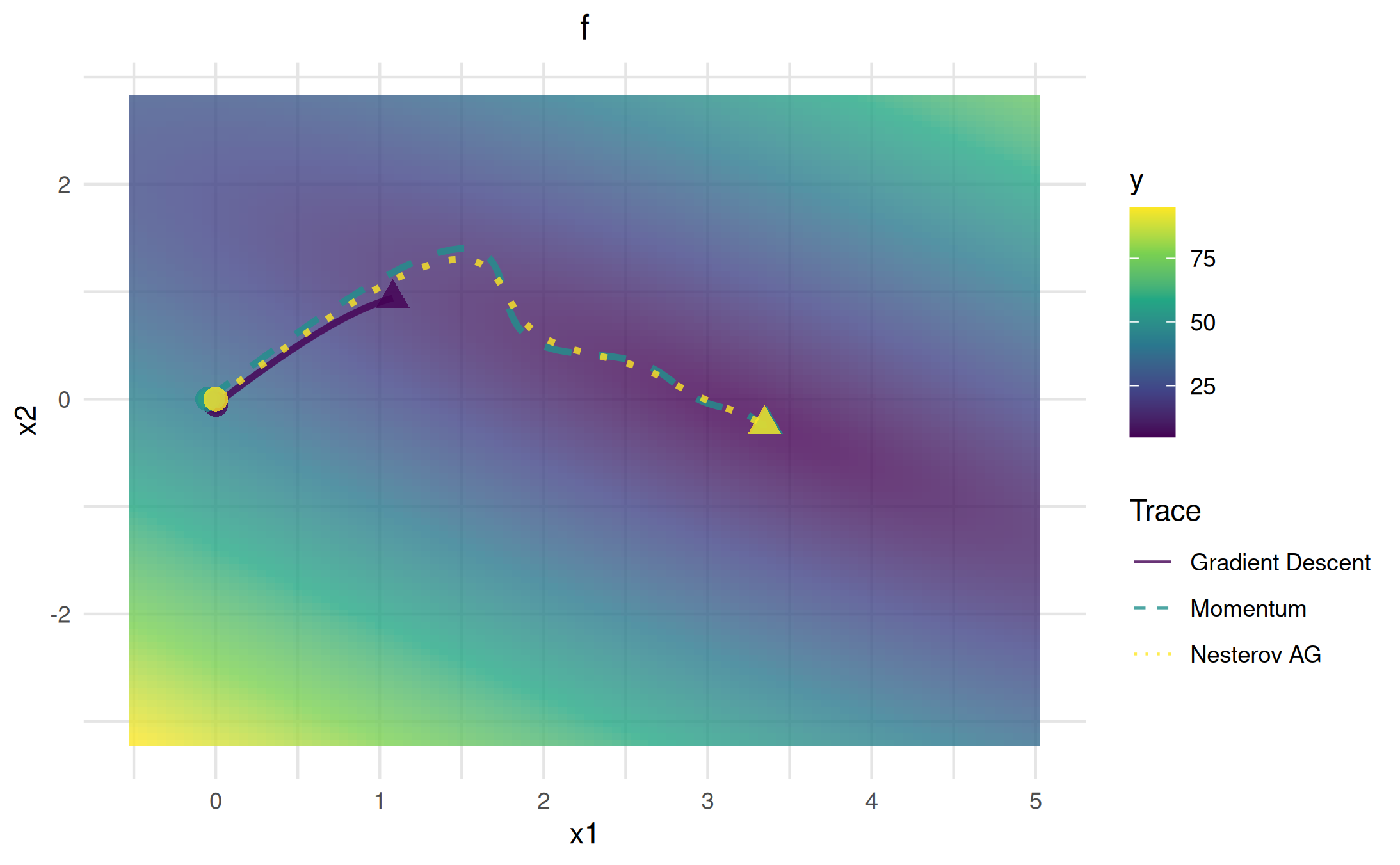
vis$plot()We can also use the alternative ggplot2 backend:
vis_2d = as_visualizer(obj_lm, x1_limits = c(-0.5, 5), x2_limits = c(-3.2, 2.8))

vis_2d$add_optimization_trace(oo1, name = "Gradient Descent")
vis_2d$add_optimization_trace(oo2, line_type = "dashed", name = "Momentum")
vis_2d$add_optimization_trace(oo3, line_type = "dotted", name = "Nesterov AG")

vis_2d$plot()