Visualization of Loss Functions • vistool

library(vistool)
options(vistool.theme = vistool_theme(
  palette = "plasma"
))

Loss functions are wrapped in LossFunction objects. The package includes predefined loss functions for both regression and classification tasks. Classification loss functions can work with different input scales (scores vs. probabilities).

as.data.table(dict_loss)
#> Key: <key>
#>                     key                    label task_type
#>                  <char>                   <char>    <char>
#>  1:               brier              Brier Score   classif
#>  2:              cauchy              Cauchy Loss      regr
#>  3:       cross-entropy            Logistic Loss   classif
#>  4: epsilon-insensitive Epsilon-Insensitive Loss      regr
#>  5:               hinge               Hinge Loss   classif
#>  6:               huber               Huber Loss      regr
#>  7:               l1_ae        L1 Absolute Error      regr
#>  8:               l2_se         L2 Squared Error      regr
#>  9:         log-barrier         Log-Barrier Loss      regr
#> 10:            log-cosh            Log-Cosh Loss      regr
#> 11:             pinball             Pinball Loss      regr

To get a loss function from the dictionary, use the lss() function. Many loss functions support parameters (e.g., quantile for pinball loss, delta for Huber loss, epsilon for epsilon-insensitive loss). You can specify these parameters directly in the lss() function call. Here we retrieve the pinball loss function for regression with a custom quantile parameter.

loss_function = lss("pinball", quantile = 0.3)

Visualization

To visualize a loss function, use the as_visualizer() function. For regression losses, the input represents residuals $r = y - f(x)$ . For classification losses, the input can be either margins $y \cdot f(x)$ (score-based) or probabilities $\pi$ (probability-based). By default, loss functions are plotted with 1000 points for smooth curves.

vis = as_visualizer(loss_function, y_pred = seq(-4, 4), y_true = 0)

Use the plot() method to plot the loss function.

vis$plot()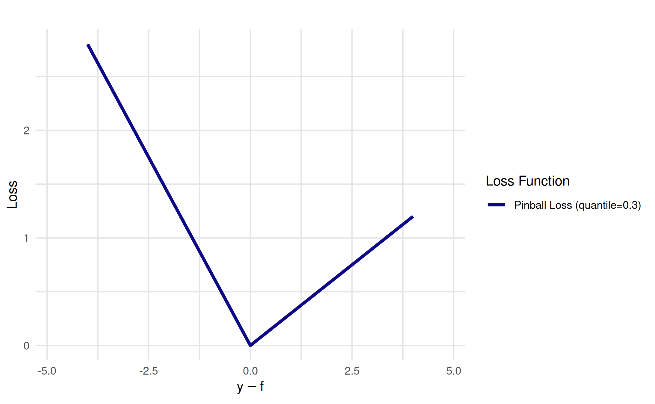

Regression Loss Functions

Here we visualize multiple regression loss functions:

loss_huber = lss("huber")
loss_l2 = lss("l2_se")
loss_l1 = lss("l1_ae")
loss_logcosh = lss("log-cosh")

vis_combined = as_visualizer(
  list(loss_huber, loss_l2, loss_l1, loss_logcosh),
  y_pred = seq(-4, 4),
  y_true = 0,
  n_points = 5000L # higher resolution for smooth curves
)
vis_combined$plot()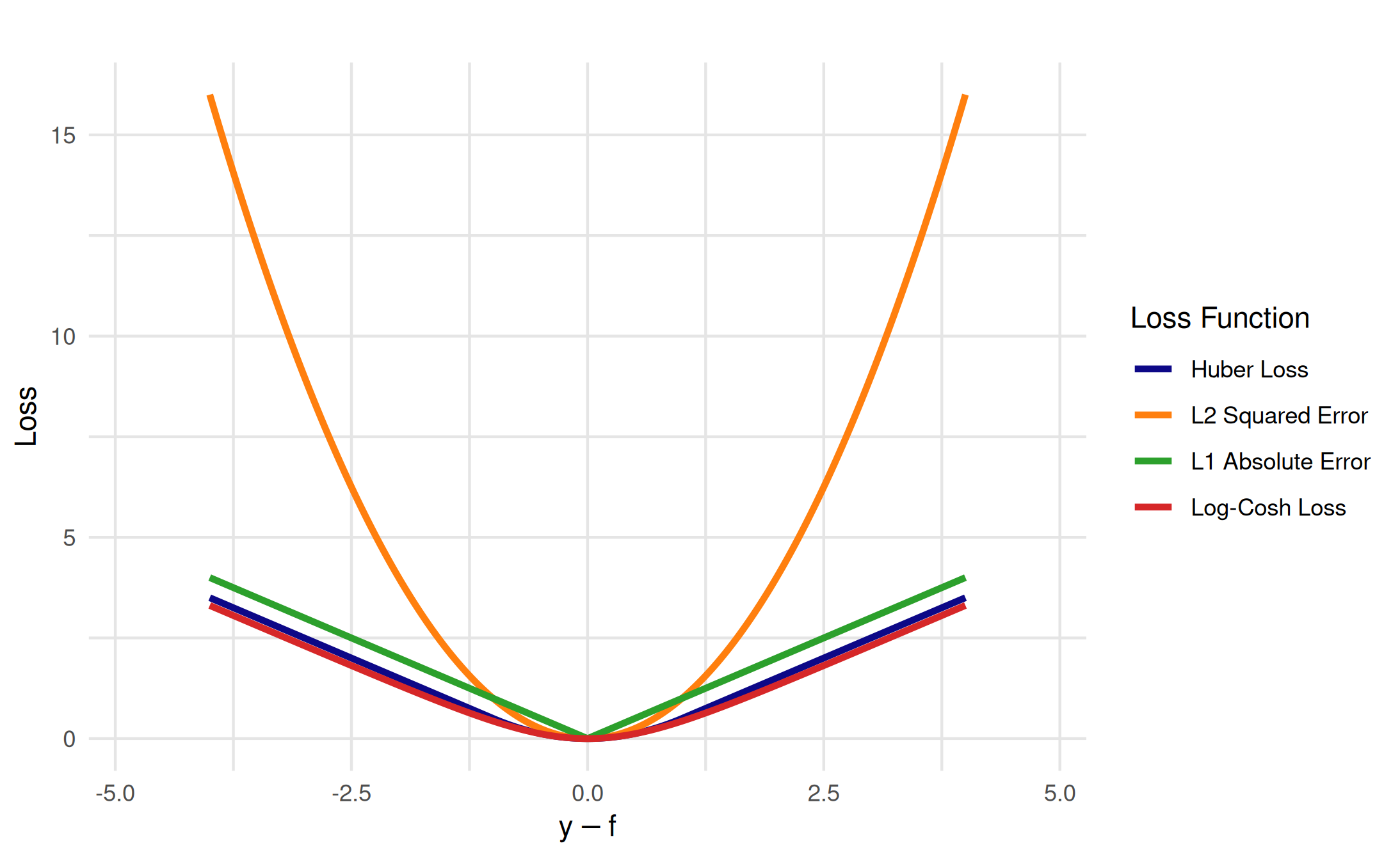

Classification Loss Functions

Classification loss functions can operate on different input scales depending on the loss function. Some work with scores, while others work with probabilities.

Score-based Classification Losses

Score-based losses operate on the margin $y \cdot f(x)$ where $y \in \{-1, +1\}$ and $f(x)$ is the prediction score:

hinge_loss = lss("hinge")
crossentropy_loss = lss("cross-entropy")

vis_scores = as_visualizer(
  list(hinge_loss, crossentropy_loss),
  input_type = "score"
)
vis_scores$plot()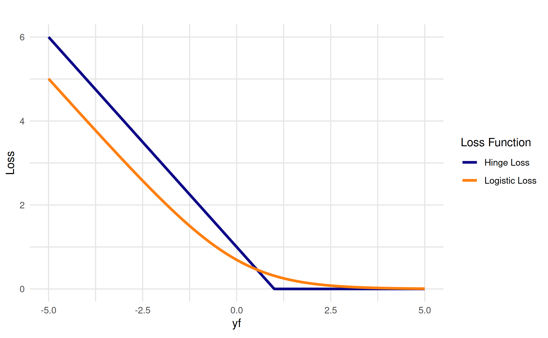

Probability-based Classification Losses

Probability-based losses operate on predicted probabilities $\pi \in [0, 1]$ . The cross-entropy loss can be expressed in both score and probability forms, while the Brier score is naturally probability-based:

brier_loss = lss("brier")

vis_probs = as_visualizer(
  list(crossentropy_loss, brier_loss),
  input_type = "probability"
)
vis_probs$plot()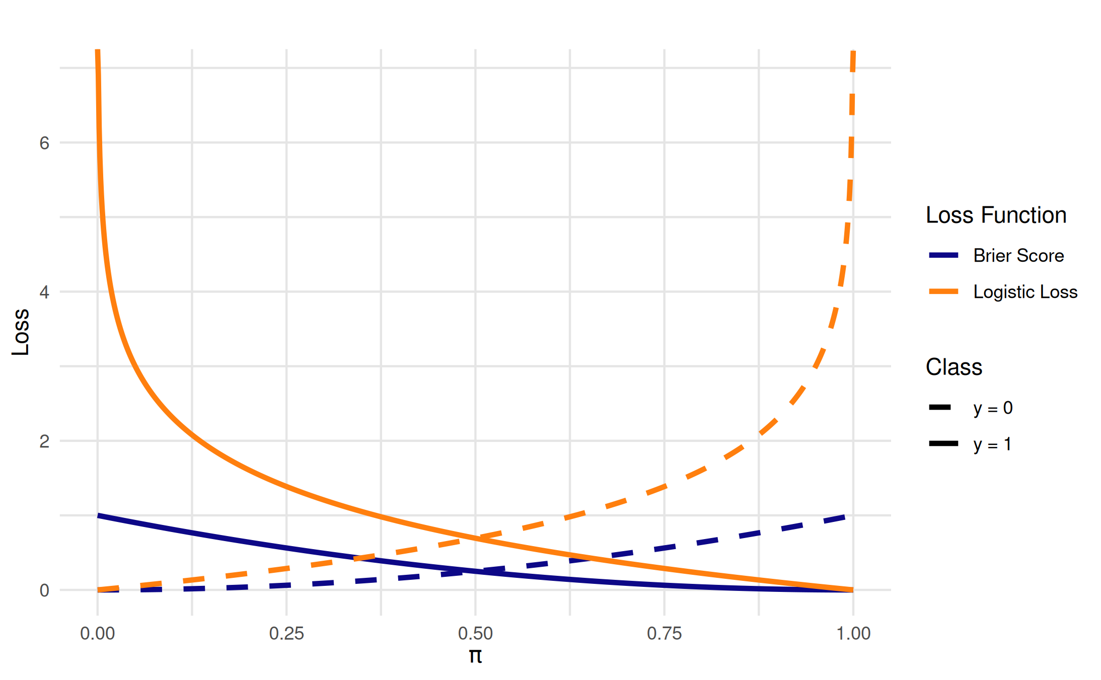

Controlling Which Class Curves to Display

When visualizing probability-based losses, you can control whether to show curves for the positive class (y = 1), negative class (y = 0), or both (default) using the y_curves parameter:

vis_y1 = as_visualizer(
  list(crossentropy_loss, brier_loss),
  input_type = "probability"
)
vis_y1$plot(y_curves = "y1") # Only show y = 1 curve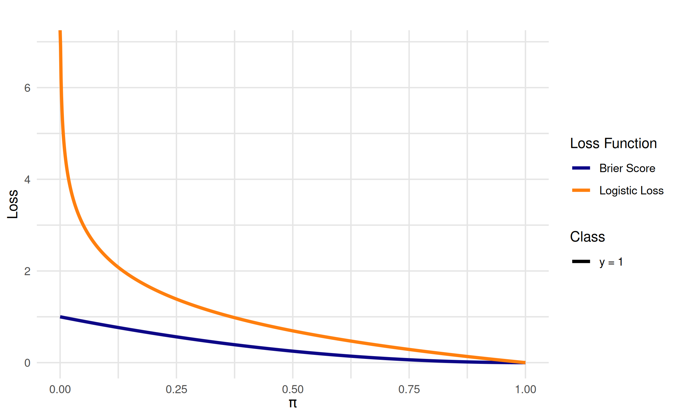

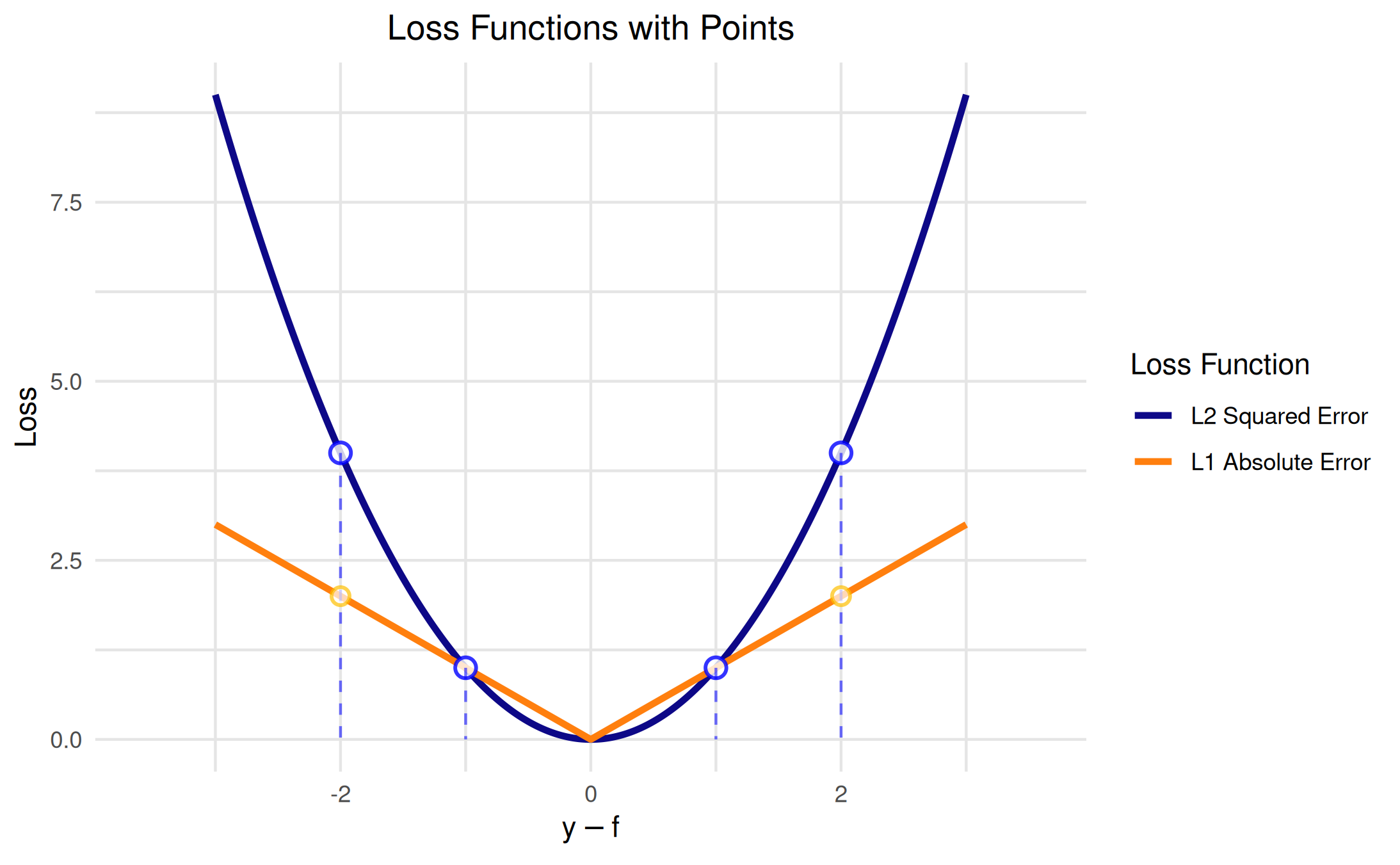
Adding Points to Loss Function Visualizations

You can add specific points to loss function plots to highlight particular residual values and their corresponding loss values. The add_points() method automatically calculates the y-coordinates by evaluating the loss function at the given x-coordinates.

vis_with_points = as_visualizer(
  list(loss_l2, loss_l1),
  y_pred = seq(-3, 3),
  y_true = 0
)

vis_with_points$add_points(
  x = c(-2, -1, 1, 2),
  loss_id = "l2",
  show_line = TRUE,
  color = "blue",
  size = 3,
  alpha = 0.8
)$add_points(
  x = c(-2, 2),
  loss_id = "l1", # Specify the L1 loss
  show_line = FALSE,
  color = "#febf01",
  size = 2.5,
  alpha = 0.7
)

vis_with_points$plot(
  plot_title = "Loss Functions with Points",
  show_legend = TRUE
)

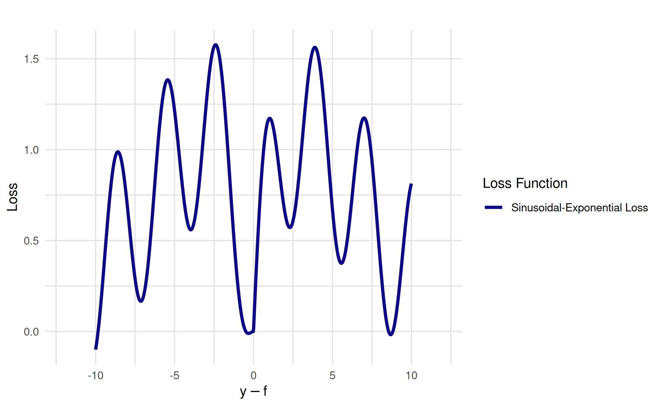
Custom Loss Functions

We can also define and visualize custom loss functions:

custom_loss = LossFunction$new(
  id = "custom_loss",
  label = "Sinusoidal-Exponential Loss",
  task_type = "regr",
  fun = function(r) abs(r) * exp(-abs(r) / 3) + 0.5 * sin(2 * r)
)

vis = as_visualizer(custom_loss, y_pred = seq(-10, 10), y_true = 0, n_points = 5000L)
vis$plot()