Advanced visualization

library(vistool)
library(plotly)
library(purrr)
set.seed(1)

This vignette covers advanced visualization options, overlays, manual layers, and animations. It complements the core vignettes and focuses on fine control and composition.

Surface visualization options

You can customize the appearance using the theme system:

vis = as_visualizer(obj("TF_franke"), type = "surface")
vis$plot(theme = list(palette = "grayscale"))

The add_contours() method allows you to add custom contour lines to the surface:

llower = vis$objective$limits_lower
lupper = vis$objective$limits_upper
ssize = (lupper - llower) / 10

vis$add_contours(contours = list(
  y = list(show = TRUE, start = llower[2], end = lupper[2], size = ssize[2], color = "red")
))$plot(theme = list(palette = "grayscale"))

Setting the layout and scene

You can customize layout and scene directly in the plot() method:

vis = as_visualizer(obj("TF_franke"), type = "surface")
vis$plot(layout = list(
  title = list(text = "Custom Title", font = list(size = 20)),
  showlegend = TRUE
))

vis$plot(scene = list(camera = list(eye = list(x = 1.5, y = 1.5, z = 1.5))))

View presets via `set_scene()`

For repeated exploration, you can set camera presets using the helper method set_scene() and then render.

vis = as_visualizer(obj("TF_branin"), type = "surface")
# classic three-quarter view
vis$set_scene(x = 1.3, y = 1.2, z = 1.0)
vis$plot()

# top-down shallow angle
vis$set_scene(x = 0.7, y = 0.7, z = 2.0)
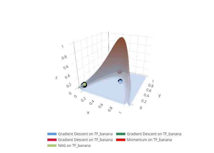
vis$plot()

Overlays: Taylor and Hessian

obj = obj("TF_banana")
# Use surface visualizer for Taylor/Hessian overlays
vis = as_visualizer(obj, type = "surface")

# Point of expansion (choose a point of interest)
x0 = c(0.85, 0.47)

# First-order Taylor plane with compact extent and visible grid contours
vis$add_taylor(
  x0,
  degree = 1,
  npoints_per_dim = 11,
  x1margin = 0.3,
  x2margin = 0.3,
  contours = list(
    x = list(show = TRUE, start = 0, end = 1, size = 0.03, color = "black"),
    y = list(show = TRUE, start = 0, end = 1, size = 0.03, color = "black")
  )
)

# Add Hessian eigen-directions anchored at x0
vis$add_hessian(x0, x1length = 0.25, x2length = 0.25)
vis$plot()

# Second-order Taylor surface (narrow z-limits for clarity)
vis2 = as_visualizer(obj, type = "surface")
vis2$add_taylor(
  x0,
  degree = 2,
  npoints_per_dim = 21,
  x1margin = 0.35,
  x2margin = 0.35,
  zlim = range(vis2$zmat, na.rm = TRUE)
)
vis2$add_hessian(x0, x1length = 0.25, x2length = 0.25)
vis2$plot()

Manual layers

You can extend the returned plot objects directly:

ggplot2: modify the ggplot result with standard layers and themes

vis2d = as_visualizer(obj("TF_franke"))
p = vis2d$plot(show_title = FALSE)
p + ggplot2::labs(title = "Franke Function") + ggplot2::theme_minimal()

plotly: add traces or update layout/scene

vis3d = as_visualizer(obj("TF_branin"), type = "surface")
p = vis3d$plot()
plotly::add_markers(p, x = c(0.5), y = c(0.5), z = c(0.0), name = "mark")

obj = obj("TF_banana")
vis = as_visualizer(obj, type = "surface")
vis$set_theme(vistool_theme(alpha = 0.5))
p = vis$plot()

# Create some synthetic points to overlay as 3D markers
nsim = 100
grid = data.frame(x = runif(nsim), y = runif(nsim))
grid$z = apply(grid, 1, vis$objective$eval) + rnorm(nsim, sd = 0.05)

# Add manual plotly layer on top of vistool’s plotly object
p %>% add_trace(
  data = grid, x = ~x, y = ~y, z = ~z, mode = "markers",
  type = "scatter3d",
  marker = list(symbol = "diamond", size = 3, color = "#2c7fb8", opacity = 0.7),
  name = "samples"
)

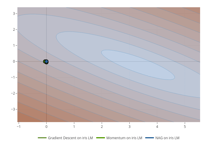
Animations

You can animate surface views and optimization traces. The code below creates frames and saves them as images; combine them into GIFs with ImageMagick.

obj = obj("TF_GoldsteinPriceLog")
oo = OptimizerGD$new(obj, x_start = c(0.22, 0.77), lr = 0.01)
oo$optimize(steps = 30)

vis = as_visualizer(obj, type = "surface")
vis$add_optimization_trace(oo)

dir.create("animation", showWarnings = FALSE)
vis$animate(
  dir = "animation",
  nframes = 20,
  view_start = list(x = 1.2, y = 1.2, z = 1.1),
  view_end   = list(x = 1.8, y = 1.4, z = 1.3),
  fext = "png",
  width = 600, height = 500
)

# Then assemble with ImageMagick, e.g.:
# convert -delay 15 -loop 0 animation/*.png optim.gif