Chapter 4 Further Topics
Authors: Marco Moldovan, Rickmer Schulte, Philipp Koch
Supervisor: Rasmus Hvingelby
So far we have learned about multimodal models for text and 2D images. Text and images can be seen as merely snapshots of the sensory stimulus that we humans perceive constantly. If we view the research field of multimodal deep learning as a means to approach human-level capabilities of perceiving and processing real-world signals then we have to consider lots of other modalities in a trainable model other than textual representation of language or static images. Besides introducing further modalities that are frequently encountered in multi-modal deep learning, the following chapter will also aim to bridge the gap between the two fundamental sources of data, namely structured and unstructured data. Investigating modeling approaches from both classical statistics and more recent deep learning we will examine the strengths and weaknesses of those and will discover that a combination of both may be a promising path for future research. Going from multiple modalities to multiple tasks, the last section will then broaden our view of multi-modal deep learning by examining multi-purpose modals. Discussing cutting-edge research topics such as the newly proposed Pathways, we will discuss current achievements and limitations of the new modeling that might lead our way towards the ultimate goal of AGI in multi-modal deep learning.
4.1 Including Further Modalities
Author: Marco Moldovan
Supervisor: Rasmus Hvingelby
Over the course of the previous chapters, we have introduced the basics of computer vision (CV) and natural language processing (NLP), after that we have learned about several directions of how we can combine these two subfields in machine learning. In the most general sense, we have explored ways in which we can process more than just one modality with our machine learning models.
So far, we have established the basics of multimodal deep learning by examining the intersection of these two most well-understood subfields of deep learning. These fields provide us with easy-to-handle data as seen in the corresponding previous chapter as well as a plethora of established and thoroughly examined models.
In reality though, text and images can be seen as only discrete snapshots of our continuous highly multimodal world. While text and images serve as an important foundation for us to develop concepts and algorithms for multimodal learning, they only represent a small part of what we as humans can perceive. First and foremost, we perceive reality in a temporal direction too, for a machine this could mean receiving video as input instead of just still images (IV, Kapoor, and Ghosh 2021). In fact, as videos are some of the most abundant types of data, we will later see that self-supervised learning on raw video is one of the major subtasks of multimodal deep learning. Clearly our reality is not just a sequence of RGB images though: just like in most videos we experience sound and speech which we would also like our models to process. Furthermore, we have different senses that can perceive depth, temperature, smell, touch, and balance among others. We also have sensors that can detect these signals and translate them to a digital signal so it is reasonable to want to have a machine learning algorithm detect and understand the underlying structure of these sensory inputs as well.
Now it might be tentative to simply list all different types of signals that we have developed sensors for and give a few examples of a state of the art (SOTA) deep neural network for each that tops some arbitrary benchmark. Since we are talking about multimodal learning, we would also have to talk about how these different modalities can be combined, and what the current SOTA research is, on all of these permutations of modalities. Quickly we would see that this list would get extremely convoluted and that we would not see the end of it. Instead of basing our understanding simply on a list of modalities we need a different, more intuitive system that lets us understand the multimodal research landscape. In the first part of this chapter we will attempt to introduce such a taxonomy based on challenges rather than modalities (Baltrušaitis, Ahuja, and Morency 2017).
If we consider multimodal deep learning as the task to learn models that can perceive our continuous reality just as precisely (if not more) than us humans (LeCun 2022), we have to ask ourselves how we can generalize our learnings from image-text multimodal learning to more types of signals. We have to ask what constitutes a different type of signal for us versus for a machine. What types of representation spaces we can learn if we are faced with having to process different signal types (modalities) and what are the strategies to learn these representation spaces. Here we will see that in large we can have two ways of processing modalities together, where defining their togetherness during training and inference will play the central role. After formalizing the types of multimodal representation learning we will move on and elaborate what the fundamental strategies are that allow is to learn these representation spaces. Then again, we can ask what we can practically do with these representation spaces: Here the notion of sampling and retrieving from our learnt representation spaces will play a major role. In fact we will see that almost all practical multimodal tasks can be generalized to what we call multimodal translation, where given a signal in one modality we want to return a semantically related signal in another modality.
The ideas that were just introduced are in fact what we consider to be the central challenges of multimodal learning, these challenges constitute the main pillars of our taxonomy of multimodal deep learning. Every problem in multimodal learning will have to solve at least one of these challenges. By viewing multimodal deep learning through these lens we can easily come across a new modality and understand immediately how to approach this problem without breaking our taxonomy.
After understanding these challenges the reader will hopefully take home a new way of thinking about how to solve and understand multimodal problems. Hopefully, when coming across a new research paper and tackling a new research project the reader will identify the challenges that the paper is trying to solve or which challenge requires solving for the research project and immediately know where to look.
Looking at the broader spectrum of the AI research landscape, as Yann LeCun has done in his recent paper (LeCun 2022), we can see that multimodal perception through deep learning is one particularly important building block for creating autonomous agents capable of displaying reason.
After having thoroughly introduced these central multimodal learning challenges we will look at some of the current research trends of multimodal deep learning from the point of view of our challenge taxonomy. In order to solve these challenges a system must implement two major building blocks: a multimodal model architecture and a training paradigm. In this part of the chapter we will introduce examples for both and successively generalize these concepts. By introducing more and more universal and problem- as well as modality-agnostic systems from current research we will lead into a research project that we ourselves are undertaking to merge a general multimodal model with a problem-agnostic training paradigm which will form the conclusion of this chapter. Hopefully by then two major concepts have transpired: 1) Introduce models and training paradigms that are general enough as to give a conclusion to this chapter’s very title: learning from any and including an arbitrary amount of further modalities in our learner and 2) sticking to the analogy of the human perceptive system and presenting models and training paradigms that can learn from any type of input signal just like we humans can. In the spirit of Yann LeCun’s JEPA paper the perceptive aspect of artificial intelligence is only one aspect of the system. Looking at the broader spectrum of the AI research landscape – as Yann LeCun has done in his recent paper, we can identify that multimodal perception through deep learning is one particularly important building block for creating autonomous agents capable of displaying reason. Other aspects such as reasoning and especially multi-tasking and scaling will be elaborated in [this] following chapter.
4.1.1 Taxonomy of Multimodal Challenges
In this part we will introduce a taxonomy based on challenges within multimodal learning (Baltrušaitis, Ahuja, and Morency 2017).
4.1.1.1 Multimodal Representation Learning
At the core of most deep learning problems lies representation learning: learning an expressive vector space of distributed embedding vectors in which we can define a distance function that informs us about the semantic relatedness of two data points in this learnt vector space. For the sake of simplicity, we will assume that these vector spaces are learnt via deep neural networks trained with backpropagation. Normally we will have to apply some preprocessing to our raw data in order to transform it into a format that a neural network can read, usually in the form of a 2-dimensional matrix. As output the neural network will return some high-dimensional vector. But what if we are presented with more than one signal type (i.e., multimodal input)? How do we structure our input so that our models can sensibly learn from this multimodal input?
![Joint and coordinated multimodal representations[@baltrušaitis2017multimodal].](figures/03-01/joint-coordinated.png)
FIGURE 4.1: Joint and coordinated multimodal representations(Baltrušaitis, Ahuja, and Morency 2017).
In the introduction for this chapter, we briefly mentioned the togetherness of multimodal signals during training and inference (Bengio, Courville, and Vincent 2013). By virtue of having more than one modality present as input into our learner – whether it be during training or inference – we want to relate these modalities somehow, this is the essence of multimodal learning. If we consider that our input signals from different modalities are somehow semantically related, we would like to leverage this relatedness across modalities and either have our learner share information between modalities and leverage this relatedness. Therefore cross-modal information has to come together at some point in our training and/or inference pipeline. How and when this happens is the central question of multimodal representation learning which we describe in this subchapter.
First, we have to specify that what is meant by their togetherness during training and inference. Togetherness loosely means that unside our learner we “merge” the information of the modalities.
To make this more concrete: on one side we could think of concatenating the input from different modalities together to form one single input matrix. This joint input then represents a new entity that consists of multiple modalities but is treated as one coherent input. The model then learns one representation for the joint multimodal signal. On the other hand, we could think of the input always as strictly unimodal for one specific model. Each model would be trained on one modality and then the different modalities are brought together only in the loss function in such a way as to relate semantically similar inputs across modalities. To formalize what we just introduced, joint representation learning refers to projecting a concatenated multimodal input into one representation space while coordinated representation learning will learn different representation spaces for each modality and coordinate them such that we can sensibly align these representation spaces and apply a common distance function that can relate points across modalities to each other.
4.1.1.1.1 Joint Representations
Given for example a video that consist of a stream of RGB images and a stream of audio signals as a waveform we would like our model to learn a representation of this whole input video as how it appears “in the wild.” Considering the entirety of the available input means that our model could leverage cross-modal information flow to learn better representations for our data: this means the model learns to relate elements from one modality to elements of the other. Of course, one could imagine concatenating all sorts of modalities together to feed into a model, such as audio and text, RGB image and depth maps, or text and semantic maps. The underlying assumption simply has to be that there is something to relate between the modalities – in other words there has to be a sensible semantic relationship between the modalities.
4.1.1.1.2 Coordinated Representation
When we are given data in multiple modalities, for learning coordinated representations, the underlying assumption will be that there exists some semantic relation between a signal in modality m and modality n. This relation can be equivalence – as in a video dataset where the audio at a given timestep t is directly intertwined with the sequence of RGB images at that timestep: they both are stand-ins for conceptually the same entity. The relation can also be a different function such as in the problem of cross-modal speech segment retrieval: here we want to return a relevant passage from an audio or speech file given a textual query. The text query is not the exact transcript of the desired speech segment, but they do relate to each other semantically, for this our model would have to learn this complex relationship across modalities (Baltrušaitis, Ahuja, and Morency 2017).
To do this we learn a class of models where each model will learn to project one modality into its own representation space. We then have to design a loss function in such a way as to transfer information from one representation to another: we essentially want to make semantically similar data points sit close together in representation space while having semantically dissimilar points sit far away from each other. Since each modality lives in its own representation space our loss function serves to align – or coordinate – these vector spaces as to fulfill this desired quality.
After having introduced what representation spaces we want to learn in the sections multimodal fusion and multimodal alignment we will elaborate further on exactly how we can learn joint and coordinate multimodal representation spaces respectively.
4.1.1.2 Multimodal Alignment
Alignment occurs when two or more modalities need to be synchronized, such as matching audio and video. It deals with the how rather than the what of learning coordinated representation spaces. Here, the goal is to learn separate representation spaces for each present modality, given that a dataset of corresponding data n-tuples exist. The embedding spaces are technically separate but through a carefully chosen learning strategy they are rotated and scaled such that their data points can be compared and queried across representation spaces. Currently the most common learning paradigm for alignment is contrastive learning. Contrastive learning was described extensively in a previous chapter, so in short: given a pair of semantically equivalent samples in different modalities we would want these data points to be as close as possible in embedding space while being far apart from semantically dissimilar samples(Baltrušaitis, Ahuja, and Morency 2017).
4.1.1.3 Multimodal Fusion
![Different types of multimodal fusion[@baltrušaitis2017multimodal].](figures/03-01/fusion.png)
FIGURE 4.2: Different types of multimodal fusion(Baltrušaitis, Ahuja, and Morency 2017).
Analogous to alignment, multimodal fusion describes how joint representations are learnt. Fusion describes the process of merging modalities inside the model, usually a concatenated and tokenized or patched multimodal input is fed into the model as a 2D matrix. The information from the separate modalities have to combine somehow inside the model to learn from one another to produce a more meaningful, semantically rich output. In the context of Transformer (Vaswani, Shazeer, Parmar, Uszkoreit, Jones, Gomez, et al. 2017c) based models this usually means where the different inputs start attending to one another cross-modally. This can happen either early on in the model, somewhere in the middle, close to the output in the last layer(s) or based on a hybrid approach. These techniques are usually either based on heuristics, the researcher’s intuition, biological plausibility, experimental evidence, or a combination of all (Nagrani et al. 2021)[@ DBLP:journals/jstsp/ZhangYHD20][@ shvetsova2021everything].
4.1.1.4 Multimodal Translation
![Different types of multimodal translation [@baltrušaitis2017multimodal].](figures/03-01/translation.png)
FIGURE 4.3: Different types of multimodal translation (Baltrušaitis, Ahuja, and Morency 2017).
In many practical multimodal use-cases we actually want to map from one modality to another: As previously mentioned we might want to return a relevant speech segment from an audio file given a text query, we want to return a depth map or a semantic map given an RGB image or we want to return a description of an image to read out for visually impaired people(Bachmann et al. 2022). In any way we are presented with a datapoint in one modality and want to translate it to a different modality. This another one of the main challenges of the multimodal deep learning landscape and it is what this subsection will be about (Sulubacak et al. 2020).
4.1.1.4.1 Retrieval
In order to perform cross-modal retrieval one essentially has to learn a mapping that maps items of one modality to items of another modality. Practically this means aligning separate unimodal representation spaces so that the neighborhood of one datapoint contains and equivalent datapoint of a different modality when its representation space is queried at that point (Shvetsova et al. 2021)[@ DBLP:conf/eccv/Gabeur0AS20].
Currently cross-modal retrieval is almost exclusively learnt via contrastive learning which we described previously (T. Chen, Kornblith, Norouzi, and Hinton 2020b)[@ oord2018representation][@ DBLP:conf/icml/ZbontarJMLD21].
4.1.1.4.2 Generation
We might also be presented with the case where we have a query in one modality but a corresponding datapoint in a different modality simply does not exist. In this case we can train generative multimodal translation models that learn to decode samples from a vector space into an output of a different modality. This requires us to learn models with a deep understanding of the structure of our data: when sampling datapoint from our cross-modal representation space and applying a decoder to produce the intended output we need to sample from a relatively smooth distribution (C. Zhang et al. 2020). Since we are actually doing interpolation between known points of our data distribution, we want to produce sensible outputs from “in between” our original data. Learning this smooth distribution often requires careful regularization and appropriate evaluation poses another challenge(Baltrušaitis, Ahuja, and Morency 2017).
With the hype around generative multimodal models created mostly by models such as Dall-E (Ramesh, Pavlov, et al. 2021c) came a huge spike in research around this area (Saharia et al. 2022a)[@ wu2022nuwainfinity]. Currently lots of models generate photorealistic outputs through diffusion (Ho, Jain, and Abbeel 2020b), yet they still employ models such as a pretrained CLIP (Radford, Kim, Hallacy, Ramesh, Goh, Agarwal, Sastry, Askell, Mishkin, Clark, Krueger, et al. 2021b) module as the backbone.
4.1.2 Current Research Trends: Generalized Self-Supervised Multimodal Perception
So far, we have understood the challenges we are faced with when trying to solve multimodal learning problems. We have understood that from a theoretical perspective we need to learn one or several semantic representation spaces and what the overarching constraints are for learning these vector spaces. Moreso, we have seen that given a coordinated representation space we can translate between modalities and decode our vector space into new data points. For joint representation spaces we can apply traditional downstream tasks such as classification or regression to better solve real world problems leveraging the interplay of all modalities at hand. Going forward we will explore the two major building blocks for realizing these challenges from a more practical perspective:
- Multimodal Architectures
- Multimodal Training Paradigms
A combination of carefully chosen model architecture and training scheme is necessary to solve the challenges we have described on a high level. Throughout the rest of this subchapter, we will look at more and more general concepts for each of these components. In this subchapter we will also connect back to one central principal that we have introduced earlier in this chapter: approaching human-level of multimodal perception. This means that we will follow one of the major lines of research within multimodal deep learning: building more general and problem-agnostic solutions. We pose the question: Why apply hyper-specific solutions when we can simplify and generalize our methods while retaining (or even improving) on experimental results. Towards the end of the chapter, we will also briefly introduce our own research in which we attempt to combine a modality agnostic model architecture with a generalized non-contrastive training paradigm for uni- and multi-modal self-supervised learning.
4.1.2.1 General Multimodal Architectures
First, we want to establish some desirable characteristics that our generalized multimodal model architectures should have:
- Input-Agnosticism: Whether our input consist of 1-dimensional sequences of audio waveforms or text or 3-dimensional inputs such as video we want out model to process all kinds of modalities equally with as little adjustments as possible.
- Multimodal Fusion: Ideally, we would also like to feed a concatenated input of several modalities into the model to learn joint representations.
- Preservation of Locality
- Respect Compositionality
- Flexible outputs: The model produces not only scalar or vector outputs but can ideally decode into any arbitrary output, thereby essentially having the capability for multimodal translation integrated.
We have not explicitly listed multimodal alignment as a desirable characteristic because the capability to perform alignment becomes trivial since we included the point about flexible outputs: to do alignment we need our model to output vectors that we can predict or regress over via a loss function. To illustrate the state of current research we will briefly introduce three multimodal model architecture that fulfill some, if not all of the above-mentioned criteria.
4.1.2.1.1 NÜWA
![Data being represented in the NÜWA-imposed 3D format[@wu2021nwa].](figures/03-01/nuwa.png)
FIGURE 4.4: Data being represented in the NÜWA-imposed 3D format(Wu et al. 2021).
Initially conceived as a generative multimodal translation model here we are especially interested in the 3D-Nearby-Attention encoder-decoder stack at the center of NÜWA (Neural visUal World creAtion). We assume that our input, whether it be 1-dimensional sequences like text (or audio, although it was not used in the paper), 2-dimensional matrices like RGB images, sketches or semantic maps or 3-dimensional matrices like video (or possibly other modalities, e.g., depth maps) is already tokenized or divided into vectorized patches in case of 2D or 3D inputs. This is simply because we are using Transformer based encoder/decoder modules, therefore we need to reduce the input size beforehand. In the case of images or video this is done by a VQ-VAE. In principle any input is in the shape of a 3D matrix where one axis represents the temporal dimensions and the other axis representing the height and width. Clearly videos would fill out this input format in every direction, for still images the temporal dimension is simply one and for sequences such as text or audio they have height and width of one respectively and only stretch along the temporal dimension. Then for every token or patch a local neighborhood is defined amongst which the self-attention mechanism is applied. This saves on computational costs as for larger inputs global self-attention between all tokens or patches can become expensive. By imposing this 3D input format on all inputs, the model preserves the geometric and temporal structure of the original inputs, together with the locality respecting 3DNA mechanism the model introduces valuable and efficient inductive biases that make the model agnostic to input modality (if it is represented in the correct format), respects locality and allows for flexible outputs as it is intended to translate from any input to arbitrary outputs. Depending on how patching is performed for input data one could imagine a setup where the 3D encoder-decoder could also implement a hierarchical structure which would also respect compositionality in data(Kahatapitiya and Ryoo 2021), but this was not studied in this paper, although a similar idea was implemented in the follow-up paper (Wu et al. 2021)[@ wu2022nuwainfinity].
4.1.2.1.2 Perceiver IO
![Perceiver encoder stack shows how the cross-attention mechanism transforms large inputs into smaller ones that can be processed by a vanilla Transformer encoder [@jaegle2021perceiver].](figures/03-01/perceiver-io.png)
FIGURE 4.5: Perceiver encoder stack shows how the cross-attention mechanism transforms large inputs into smaller ones that can be processed by a vanilla Transformer encoder (Jaegle, Gimeno, Brock, Vinyals, Zisserman, and Carreira 2021a).
The Perceiver consists of a vanilla Transformer encoder block, with the follow-up paper, Perceiver IO, adding an analogous Transformer decoder in order to produce arbitrary multimodal outputs. The trick the Perceiver introduces in order to process nearly any sort of (concatenated) multimodal input is a specific cross-attention operation. Given a (very long) input in of size \(M \times C\) a so-called latent array of size \(N\times D\) is introduced, where \(N\ll M\). With the input array acting as key and value and the latent array as the query a cross-attention block is applied between the two, this transforms the original input to a much smaller size, achieving higher than 300x compression. Perceiver IO is currently likely the most flexible model when it comes to processing and outputting arbitrary multimodal outputs, it also easily handles the learning of joint representation spaces at it can process very large input array of concatenated multimodal data such as long videos with audio or optical flow maps(Jaegle, Gimeno, Brock, Vinyals, Zisserman, and Carreira 2021b)[@ jaegle2021perceiver].
4.1.2.1.3 Hierarchical Perceiver
![The hourglass structure of the Hierarchical Perceiver (HiP)[@carreira2022hierarchical].](figures/03-01/hierarchical-perceiver.png)
FIGURE 4.6: The hourglass structure of the Hierarchical Perceiver (HiP)(Carreira et al. 2022).
With information about locality and compositionality being mostly lost in the Perceiver IO encoder this follow up paper imposes a hierarchical hourglass-like structure on the encoder-decoder stack. An input matrix with length M tokens is broken down into G groups, each M/G in size. For each group a separate latent array of size \(K \times Z\) is initialized, and a cross-attention operation is applied between each group and its respective latent array, followed by a number of self-attention + MLP blocks. The set of output vectors of each group is then merged to form an intermediary matrix consisting of KG tokens. This intermediary matrix can be used as input to the next block, forming the hierarchical structure of the encoder. Besides embedding more of the locality and compositionality of data into the model, this architecture also improves upon computational costs on comparison to Perceiver IO (Carreira et al. 2022).
4.1.2.2 Multimodal Training Paradigms
Research of the past years has shown that in deep learning usually it is best to perform some sort of generalized task-agnostic pretraining routine. During self-supervised training that does not rely on any labeled data our model is trained to find underlying structures in the given unlabeled data. Given the right modeling and training scheme the model is able to approximate the true data distribution of a given dataset. This is extremely helpful as unlabeled data is extremely abundant so self-supervised learning lends itself as a way to infuse knowledge about the data into our model that it can leverage either directly for a downstream task (zero-shot) or helps as a running start during fine-tuning.
Since the conceptual part of pre-training was shown to have such an immense influence on downstream task performance, we will mainly focus on the self-supervised learning aspect of multimodal deep learning in this subchapter.
For self-supervised multimodal training paradigms, we can devise two major subcategories: those training paradigms that are agnostic to the input modality but operate only on a unimodal input and those that are both agnostic to input modalities but are truly multimodal.
4.1.2.2.1 Uni-Modal Modality-Agnostic Self-Supervised Learning
BYOL (Grill, Strub, Altch’e, et al. 2020) has introduced a paradigm shift for uni-modal self-supervised learning with its latent prediction mechanism. Its core idea is that the model to be trained is present in a student state and a teacher state where the teacher is a copy of the student with its weights updated by an exponentially moving average (EMA) of the student. Initially, BYOL was trained only on images: two augmentations would be applied to a base image and are then fed to the student and teacher network. The student would predict the latent states of last layers the teacher network via a simple regression loss. Data2vec extends this idea by generalizing it to other modalities: instead of applying specific augmentations to a base image a masking strategy is designed for each modality in order to augment the inputs, i.e., construct a semantically equivalent altered input. In the paper each modality has its own specific masking strategy and encoder backbone but in principle the paper showed that latent prediction SSL can be applied to other modalities such as text and audio just as well. Later we will introduce our own line of research where we try to generalize and simplify this even further and apply this concept to joint and coordinated representation problems.
Data2vec (Baevski et al. 2022) has already been extensively introduced in a previous chapter, because of that we would like to focus here on the importance of this relatively new line of SSL strategy that we call latent prediction SSL and why we think it is especially suitable for multimodal problems.
![Illustration of data2vec[@baevski2022data2vec].](figures/03-01/data2vec.png)
FIGURE 4.7: Illustration of data2vec(Baevski et al. 2022).
First off, how is latent prediction training different from other major SSL strategies like contrastive learning, masked auto-encoding (MAE) or masked token prediction? Whereas MAE and masked token prediction predict or decode into data space – meaning they need to employ a decoder or predict a data distribution – latent space prediction operates directly on the latent space. This means that the model has the predict the entire embedded context of an augmented or masked input, this forces the model to learn a better contextual embedding space and (hopefully) learn more meaningful semantic representations. Compared to contrastive approaches latent prediction methods do not require any hard negatives to contrast with. This alleviates us from the problem of producing hard negatives in the first place. Usually, they are sampled in-batch at training time with nothing guaranteeing us they are even semantically dissimilar (or how much so) from the anchor. The loss function of latent prediction SSL is usually L1 or L2 regression loss which is easy and straight-forward and without the need to predict in data space or mine hard negatives we avoid many of the disadvantages of the other SSL training schemes while also improving upon contextuality of our embeddings by virtue of prediction in latent space (Baevski et al. 2022).
Since this training paradigm is generalizable to multimodal problems and avoids common points of failure of other major SSL strategies it is in line with the principle that we follow here, namely: Why solve a harder problem when we can simplify it and retain performance and generality?
4.1.2.2.2 Multimodal Self-Supervised Learning
As we have elaborated extensively, we are faced with learning either joint or coordinated representations in virtually any multimodal problem. Currently no learning framework or paradigm covers both joint and coordinated learning at the same time. Joint representations are usually learnt via contrastive methods whereas coordinated representations usually employ some variant of masked input prediction or denoising autoencoding.
As an example, for multimodal contrastive learning for joint representations we will first look at VATT (Akbari et al. 2021), short for Video-Audio-Text Transformer. In this paper the authors propose a simple framework for learning cross-modal embedding spaces across multiple (>= 2) modalities at once. They do so by introducing an extension to InfoNCE loss called Multiple-Instance-Learning-NCE (MIL-NCE). The model first linearly projects each modality into a feature vector and feeds it through a vanilla Transformer backbone. If the model is only used to contrast two modalities, then a normal InfoNCE loss is being used, for a video-audio-text triplet a semantically hierarchical coordinated space is learnt that enables us to compare video-audio and video-text by the cosine similarity. First a coordinated representation between the video and audio modality is constructed via the InfoNCE (T. Chen, Kornblith, Norouzi, and Hinton 2020b) loss. Then a coordinated representation between the text modality and the now joint video-audio modality is also constructed similarly as shown in this figure. This hierarchy in these coordinated representations is motivated by the different levels of semantic granularity of the modalities, therefore this granularity is introduced into the training as an inductive bias. The aggregation of the several InfoNCE at different levels serves as the central loss function for this training strategy. It quickly becomes evident how this principle of learning (hierarchical) coordinated embeddings spaces can serve to learn between any n-tuples of different modalities if the respective n-tuples exist in a dataset.
MultiMAE (Bachmann et al. 2022) is a different kind of paper in which the authors learn a joint representation of a concatenated input consisting of RGB images, depth, and semantic maps. The input is partitioned into patches with some of them randomly selected for masking. The flattened masked input is then fed into a multimodal ViT (Dosovitskiy et al. 2021) backbone. The authors then use different decoder blocks that act upon only the unimodal segments of the input. They hypothesize that the multimodal transformer can leverage cross-modal information in the input well enough as to embed multimodal semantic information in the output states. An additional global token that can access all input modalities is added for learning the joint representation. The task-specific decoders reconstruct their respective modality also by using one cross-attention module that can access information from the whole (multimodal) input. The aggregate reconstruction loss of all decoders serves as the model’s loss function. This training strategy thereby produces a joint representation of an arbitrary ensemble of patched 2D modalities and can simultaneously learn to perform unimodal tasks as well.
![Masking and cross-modal prediction visualized for MultiMAE[@bachmann2022multimae].](figures/03-01/multimae.png)
FIGURE 4.8: Masking and cross-modal prediction visualized for MultiMAE(Bachmann et al. 2022).
So far, we have seen that for multimodal self-supervised learning we have a class of strategy that revolves around learning coordinated representations using contrastive learning. After having met contrastive multimodal models such as CLIP in earlier chapters we have shown that we can extend the same principles to include further modalities such as audio and video. In fact, if we are provided, with collections of multimodal data that pairs one modality to another, this principle can be applied to any set of given modalities.
Also, we have met training strategies that aim to generalize joint representation learning to multiple modalities. While the presented MultiMAE focuses on 2-dimensional modalities such as RGB, depth and semantic maps we could easily imagine applying the same principle to include other modalities as well – given we can process our raw signals to represent them in the appropriate format a model can read.
We have omitted any specific learning strategies that pretrain specifically for translation tasks. For retrieval tasks it is evident that contrastive methods would offer zero-shot cross-modal retrieval capabilities. For generative tasks, the interested reader is invited to study the NÜWA paper whose 3D multimodal encoder we have introduced earlier: in it the authors leverage an identical 3D decoder to translate modalities one into another in a self-supervised manner. While the NÜWA 3D Attention encoder-decoder stack is not technically a multimodal model they do apply cross-modal cross-attention in to transfer semantic information from an encoded prompt to the decoder.
4.1.2.2.3 Personal Research: General Non-Contrastive Multimodal Representation Learning
So far, we have looked at unimodal and multimodal SSL as two separate categories. Research so far has not married the two concepts into a training paradigm that can learn both multimodal joint representations as well as cross-modal coordinated representations.
Let us consider a concatenated multimodal input signal. This concatenated input array would only really differ from a unimodal signal in that it already contains modality specific encodings added to the raw input – similar to those seen in the Perceiver. In fact, let us consider a multimodal input of the exact format seen in the Perceiver. In principle we could apply some masking strategy to this input array to mask out consecutive chunks of the input matrix and apply the same latent prediction training paradigm as seen in data2vec. We craft this masking strategy in such a way as to account for highly correlated nearby signals. If we were to randomly mask single rows of the input the task of predicting the mask input for very long inputs such as in videos or audio files becomes too trivial.
By representing all inputs, whether they are unimodal or multimodal in this unified format inspired by the Perceiver and applying a generic masking strategy we have essentially generalized data2vec to any arbitrary uni- or multimodal input. A Perceiver backbone model ensures that the handling and encoding of exceptionally large input arrays becomes efficient and effective.
Similarly let us consider a multimodal input for coordinated representations. Let us also assume that our model shares its weights across the separate modality-specific representation spaces (similar to VATT). Latent prediction training schemes such as BYOL and data2vec feed separate augmentations of the same input into the model which can be either in student or teacher (or online and offline) mode. The assumption is that both inputs should be roughly semantically equivalent so the model can learn to ignore the augmentations or masks to catch the essential structure within the data. We pose the question: Are different modalities of the same thing also not just as semantically equivalent? Can we view different modalities simply as augmentations of one another and leverage the same training paradigm as in BYOL and data2vec, feeding one modality into the student model while feeding another into the teacher model? Would this learner be able to catch the essence of semantic equivalence of these two input signals? In our research project we try to answer these questions as well, our unified generalized multimodal learning framework is the first of its kind to be applicable to both joint as well as coordinated representations without any adjustments.
We propose this unified multimodal self-supervised learning framework as a novel and first-of-its-kind training paradigm that generalizes the unimodal self-supervised latent prediction training scheme inspired by BYOL and data2vec to an arbitrary number of input modalities for joint representation learning as well as cross-modal coordinated representation learning without the use of contrastive methods. Our method requires data to be presented in a generic format proposed by the Perceiver and requires just one single masking strategy.
This resolves the need for modality-specific masking strategies and models like in data2vec. For the cross-modal use-case we eliminate the need for hard negatives which are usually required for contrastive learning.
4.2 Structured + Unstructured Data
Author: Rickmer Schulte
Supervisor: Daniel Schalk
4.2.1 Intro
While the previous chapter has extended the range of modalities considered in multimodal deep learning beyond image and text data, the focus remained on other sorts of unstructured data. This has neglected the broad class of structured data, which has been the basis for research in pre-deep learning eras and which has given rise to many fundamental modeling approaches in statistics and classical machine learning. Hence, the following chapter aims to give an overview of both data sources and will outline the respective ways how these have been used for modeling purposes as well as more recent attempts to model them jointly.
Generally, structured and unstructured data substantially differ in certain aspects such as dimensionality and interpretability. This has led to various modeling approaches that are particularly designed for the special characteristics of the data types, respectively. As shown in previous chapters, deep learning models such as neural networks are known to work well on unstructured data. This is due to their ability to extract latent representation and to learn complex dependencies from unstructured data sources to achieve state-of-the art performance on many classification and prediction tasks. By contrast, classical statistical models are mostly applied on tabular data due the advantage of interpretability inherent to these models, which is commonly of great interest in many research fields. However, as more and more data has become available to researchers today, they often do not only have one sort of data modality at hand but both structured and unstructured data at the same time. Discarding one or the other data modality makes it likely to miss out on valuable insights and potential performance improvements.
Therefore, in the following sections we will investigate different proposed methods to model both data types jointly and examine similarities and differences between those. Different fusion strategies to integrate both types of modalities into common deep learning architectures are analyzed and evaluated, thereby touching upon the concept of end-to-end learning and its advantages compared to separated multi-step procedures. The different methods will be explored in detail by referring to numerous examples from survival analysis, finance and economics. Finally, the chapter will conclude with a critical assessment of recent research for combining structured and unstructured data in multimodal DL, highlighting limitations and weaknesses of past research as well as giving an outlook on future developments in the field.
4.2.2 Taxonomy: Structured vs. Unstructured Data
In order to have a clear setup for the remaining chapter, we will start off with a brief taxonomy of data types that will be encountered. Structured data, normally stored in a tabular form, has been the main research object in classical scientific fields. Whenever there was unstructured data involved, this was normally transformed into structured data in an informed manner. Typically, doing so by applying expert knowledge or data reduction techniques such as PCA prior to further statistical analysis. However, DL has enabled unsupervised feature extraction from unstructured data and thus to feed it to the models directly. Classical examples of unstructured data are image, text, video, and audio data as shown in the figure below. Of these, image data in combination with tabular data is the most frequently encountered. Hence, this combination will be examined along various examples later in the chapter. While previously mentioned data types allow for a clear distinction, lines can become increasingly blurred. For example, the record of a few selected biomarkers or genes from patients would be regarded as structured data and normally be analyzed with classical statistical models. On the contrary, having the records of multiple thousand biomarkers or genes would rather be regarded as unstructured data and usually be analyzed using DL techniques. Thus, the distinction between structured and unstructured data does not only follow along the line of dimensionality but also concerns the interpretability of single features within the data.
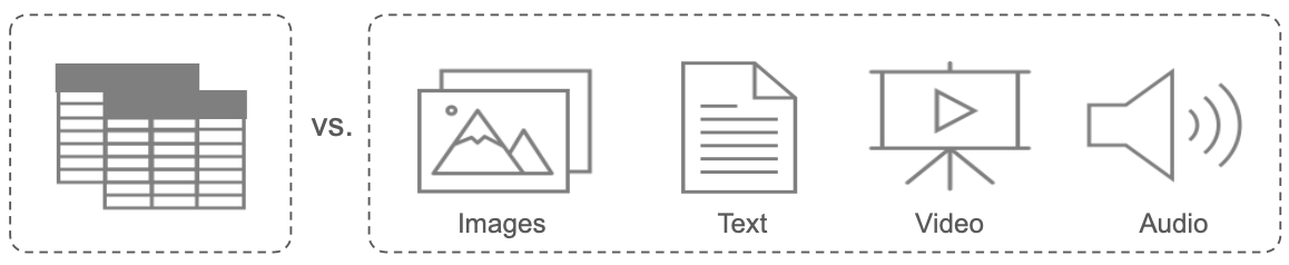
FIGURE 4.9: Structured vs. Unstructured Data
4.2.3 Fusion Strategies
After we have classified the different data types that we will be dealing with, we will now discuss different fusion strategies that are used to merge data modalities into a single model. While there are potentially many ways to fuse data modalities, a distinction between three different strategies, namely early, joint and late fusion has been made in the literature. Here we follow along the taxonomy laid out by Huang et al. (2020) with a few generalizations as those are sufficient in our context.
Early fusion refers to the procedure of merging data modalities into a common feature vector already at the input layer. The data that is being fused can be raw or preprocessed. The step of preprocessing usually involves dimensionality reduction to align dimensions of the input data. This can be done by either training a separate DNN (Deep Neural Network), using data driven transformations such as PCA or directly via expert knowledge.
Joint fusion offers the flexibility to merge the modalities at different depths of the model and thereby to learn latent feature representations from the input data (within the model) before fusing the different modalities into a common layer. Thus, the key difference to early fusion is that latent feature representation learning is not separated from the subsequent model. This allows backpropagation of the loss to guide the process of feature extraction from raw data. The process is also called end-to-end learning. Depending on the task, CNNs or LSTMs are usually utilized to learn latent feature representations. As depicted in the figure below, it is not required to learn lower dimensional feature representations for all modalities and is often only done for unstructured data. A further distinction between models can be made regarding their model head, which can be a FCNN (Fully Connected Neural Network) or a classical statistical model (linear, logistic, GAM). While the former can be desirable to capture possible interactions between modalities, the latter is still frequently used as it preserves interpretability.
Late fusion or sometimes also called decision level fusion is the procedure of fusing the predictions of multiple models that have been trained on each data modality separately. The idea originates from ensemble classifiers, where each model is assumed to inform the final prediction separately. Outcomes from the models can be aggregated in various ways such as averaging or majority voting.
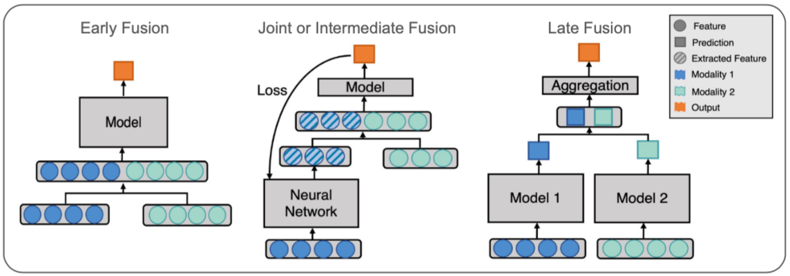
FIGURE 4.10: Data Modality Fusion Strategies (Adopted from Huang et al. 2020).
We will refer to numerous examples of both early and joint fusion in the following sections. While the former two are frequently applied and easily comparable, late fusion is less common and different in nature and thus not further investigated here. As a general note, for the sake of simplicity we will refer to the special kind of multimodal DL including both structured and unstructured data when we speak about multimodal DL in the rest of the chapter.
4.2.4 Applications
The following section will discuss various examples of this kind of multimodal DL by referring to different publications and their proposed methods. The publications originate from very different scientific fields, which is why methods are targeted for their respective use case. Hence, allowing the reader to follow along the development of methods as well as the progress in the field. Thereby, obtaining a good overview of current and potential areas of applications. As there are various publications related to this kind of multimodal DL, the investigation is narrowed down to publications which either introduce new methodical approaches or did pioneering work in their field by applying multimodal DL.
4.2.4.1 Multimodal DL in Survival
Especially in the field of survival analysis, many interesting ideas were proposed with regards to multimodal DL. While clinical patient data such as electronic health records (EHR) were traditionally used for modeling hazard functions in survival analysis, recent research has started to incorporate image data such as CT scans and other modalities such as gene expression data in the modeling framework. Before examining these procedures in detail, we will briefly revisit the classical modeling setup of survival analysis by discussing the well-known Cox Proportional Hazard Model (CPH).
4.2.4.2 Traditional Survival Analysis (CPH Model)
Survival Analysis generally studies the time duration until a certain event occurs. While many methods have been developed to analyze the effect of certain variables on the survival time, the Cox Proportional Hazard Model (CPH) remains the most prominent one. The CPH model models the hazard rate which is the conditional probability of a certain event occurring in the next moment given that it has not so far:
\[ h(t|x) = h_0(t) * e^{x\beta} \] where \(h_0(t)\) denotes the baseline hazard rate and \(\beta\) the linear effects of the covariates \(x\) on which the probability is conditioned on. The fundamental assumption underlying the traditional CPH is that covariates influence the hazard rate proportionally and multiplicatively. This stems from the fact that the effects in the so-called risk function \(f(x) = x\beta\) are assumed to be linear. Although this has the advantage of being easily interpretable, it does limit the flexibility of the model and thus also the ability to capture the full dynamics at hand.
4.2.4.3 Multimodal DL Survival Analysis
Overcoming the limitations of the classical CPH model, Katzman et al. (2018) were among the first to incorporate neural networks into the CPH and thereby replacing the linear effect assumption. While their so-called DeepSurv model helped to capture interactions and non-linearities of covariates, it only allowed modeling of structured data. This gave rise to the model DeepConvSurv of Zhu, Yao, and Huang (2016), who apply CNNs to extract information from pathological images in order to predict risk of patients subsequently. They showed that learning features from images via CNNs in an end-to-end fashion outperforms methods that relied on hand-crafting features from these images. Building on the idea of DeepConvSurv, Yao et al. (2017) extended the model by adding further modalities. Besides pathological images, their proposed DeepCorrSurv model also includes molecular data of cancer patients. The name of the model stems from the fact that separate subnetworks are applied to each modality and that the correlation between the output of these modality specific subnetworks are maximized before fine-tuning the learned feature embedding to perform well on the survival task. The correlation maximization procedure aims to remove the discrepancy between modalities. It is argued that the procedure is beneficial in small sample settings as it may reduce the impact of noise inherent to a single modality that is unrelated to the survival prediction task.
The general idea is that the different modalities of multimodal data may contain both complementary information contributed by individual modalities as well as common information shared by all modalities. The idea was further explored by subsequent research. Tong et al. (2018) for example introduced the usage of auto encoders (AE) in this context by proposing models that extract the lower dimensional hidden features of the AE applied to each modality. While their first model trains AEs on each modality separately before concatenating the learned features (ConcatAE), their second model obtains cross-modality AEs that are trained to recover both modalities from each modality respectively (CrossAE). Here, the concept of complementary information of modalities informing survival prediction separately gives rise to the first model, whereas the concept of retrieving common information inherent across modalities gives rise to the latter. Although, theoretically both models could also handle classical tabular EHR data, they were only applied to multi-omics data such as gene expressions of breast cancer patients.
Similar to Tong et al. (2018), Cheerla and Gevaert (2019) also derive their model from the idea of common information that is shared by all modalities. Besides, having specialized subnetworks for each modality to learn latent feature embeddings, they also introduce a similarity loss that is added to the classical cox loss from the survival prediction. This similarity loss is applied to each subnetwork output and aims to learn modality invariant latent feature embeddings. This is desirable not only for noise reduction but also in cases of missing data. While previous research often applied their models only on subsets of the large cancer genome atlas program (TCGA), Cheerla and Gevaert (2019) analyze 20 different cancer types of the TCGA using four different data modalities. As expanding the scope of the study increases the problem of data missingness, they specifically target the problem by introducing a variation of regular dropout, which they refer to as multimodal dropout. Instead of dropping certain nodes, multimodal dropout drops entire modalities during training in order to make models less dependent on one single data source. This enables the model to better cope with missing data during inference time. Opposed to Tong et al. (2018), the model is trained in an end-to-end manner and thus allows latent feature learning to be guided by the survival prediction loss. More impressive than their overall prediction performances are the results of T-SNE-mappings that are obtained from the learned latent feature embeddings. One sample mapping is displayed in the figure below, which nicely shows the clustering of patients with regards to cancer types. This is particularly interesting regarding the fact that the model was not trained on this variable. Besides being useful for accurate survival prediction, such feature mappings can directly be used for patient profiling and are thus pointed out as a contribution to the research on their own.
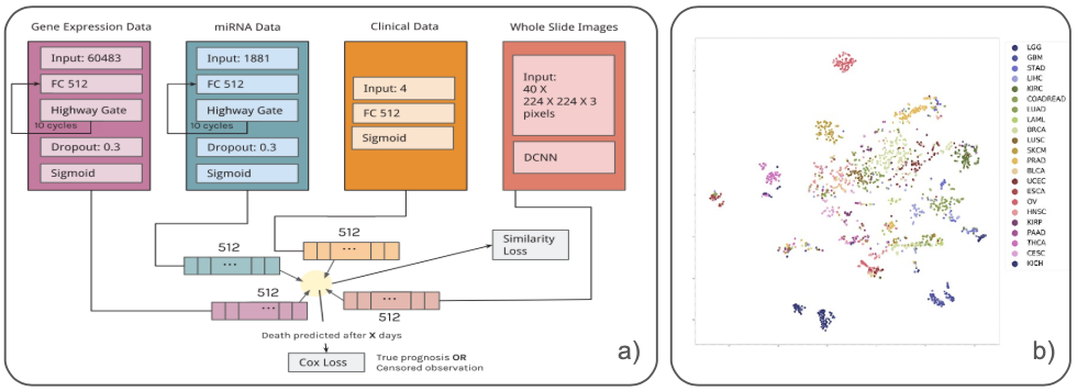
FIGURE 4.11: a) Architecture with Similarity Loss b) T-SNE-Mapped Representations of Latent Features (Colored by Cancer Type) (Cheerla and Gevaert 2019).
Vale-Silva and Rohr (2021) extend the previous work by enlarging the scope of study, analyzing up to six different data modalities and 33 cancer types of the TCGA dataset. Their so-called MultiSurv model obtains a straightforward architecture, applying separate subnetworks to each modality and a subsequent FCNN (model head) to yield the final survival prediction. Testing their modular model on different combinations of the six data modalities, they find the best model performance for the combination of structured clinical and mRNA data. Interestingly, including further modalities lead to slight performance reductions. Conducting some benchmarking, they provide evidence for their best performing model (structured clinical + mRNA) to outperform all single modality models. However, it is worthwhile mentioning that their largest model, including all six modalities, is not able to beat the classical CPH model, which is based on structured clinical data only. While this already may raise concerns about the usefulness of including so many modalities in the study, high variability of model performance between the 33 cancer types is also found by the authors and may indicate a serious data issue. The finding may seem less surprising, considering the fact that tissue appearances can differ vastly between cancer types. This is particularly problematic as for some of these cancer types only very few samples were present in the training data. For some there were only about 20 observations in the training data. Although state-of-the-art performance is claimed by the authors, the previously mentioned aspects do raise concerns about the robustness of their results. Besides, facing serious data quantity issues for some cancer types, results could simply be driven by the setup of their analysis by testing the model repeatedly on different combinations of data modalities. Thereby increasing the chances to achieve better results at least for some combinations of data modalities. Moreover, the study nicely showcases that the most relevant information can often be retrieved from classical structured clinical data and that including further modalities can by contrast even distort model training when sample sizes are low compared to the variability within the data. While these concerns could certainly have been raised for the other studies as well, they simply become more apparent in Vale-Silva and Rohr (2021) due their comprehensive and transparent analysis.
In the last part of this section we will refer to a different set of survival models by introducing the concept of Wide & Deep NN. The idea for Wide & Deep NN was first introduced by Cheng et al. (2016), who proposed to not only feed data inputs to either a linear or FCNN model part, but both at the same time. Applying it in the context of Recommender Systems, the initial assumption was that models need to be able to memorize as well as generalize for prediction tasks and that these aspects could be handled by the linear and FCNN part, respectively.
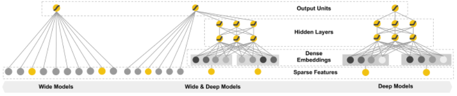
FIGURE 4.12: Illustration of Wide & Deep Neural Networks (Cheng et al. 2016).
The idea of Wide & Deep NN is applied in the context of multimodal DL survival by Pölsterl et al. (2019) and Kopper et al. (2022). Similar to previous studies Pölsterl et al. (2019) make use of the CPH model and integrate Wide & Deep NN in these. By contrast, Kopper et al. (2022) integrate them in a different set of survival models, namely the piecewise exponential additive mixed model (PAMM). The general purpose of this model class is not only to overcome the linearity but also the proportionality constraint in the classical CPH. By dropping the proportionality assumption, these models yield piecewise constant hazard rates for predetermined time intervals. Although the two studies differ in their model setup, both studies leverage structured as well as visual data and additionally make use of a linear model head. The latter is particularly interesting as it is this additive structure in the last layer of the models which preserves interpretability. Thus, they obtain models that not only have the flexibility for accurate predictions themselves but which are also able to recover the contributions of single variables to these predictions.
Although, Wide & Deep NN are advantageous due to their flexibility and interpretability, special care needs to be taken regarding a possible feature overlap between the linear and NN part as it can lead to an identifiability problem. This can be illustrated by considering the case that a certain feature \(x\) is fed to the linear as well as the FCNN model part. Because of the Universal Approximation Theorem for Neural Networks, it is known that the FCNN part could potentially model any arbitrary relation between the dependent and independent variable (\(d(x)\)). However, this is what raises the identifiability issue as the coefficients (\(\beta\)) of the linear part could theoretically be altered arbitrarily (\(\widetilde{\beta}\)) without changing the overall prediction when the weights of the NN (\(\widetilde{d}(x)\)) are adjusted accordingly.
\[ x\beta + d(x) = x\widetilde{\beta} + d(x) + f(x) = x\widetilde{\beta} + \widetilde{d}(x) \] Generally, there are two ways to deal with this identifiability problem. The first possibility would be to apply a two-stage procedure by first estimating only the linear effects and then applying the DL model part only on the obtained residuals. An alternative way would be to incorporate orthogonalization within the model, thereby performing the procedure in one step and allowing for efficient end-to-end training. The latter was proposed by Rügamer, Kolb, and Klein (2020) and utilized in the DeepPAMM model by Kopper et al. (2022). The next section will go into more detail about the two possibilities to solve the described identifiability issue and proceed by discussing further applications of multimodal DL in other scientific fields.
4.2.4.4 Multimodal DL in Other Scientific Fields
After having seen multiple applications of multimodal DL in survival analysis which predominantly occurs in the biomedical context, we will now extend the scope of the chapter by discussing further applications of multimodal DL related to the field of economics and finance. While structured data has traditionally been the main studied data source in these fields, recent research has not only focused on combining both structured and unstructured data, but also on ways to replace costly collected and sometimes scarcely available structured data with freely available and up-to-date unstructured data sources using remote sensing data. Before examining these approaches, we will first go into more detail about the model proposed by Rügamer, Kolb, and Klein (2020), which not only introduced a new model class in the context of multimodal DL but also offered a method to efficiently solve the above mentioned identifiability problem.
As previous research exclusively focused on mean prediction, uncertainty quantification has often received less attention. Rügamer, Kolb, and Klein (2020) approach this by extending structured additive distributional regression (SADR) to the DL context. Instead of learning a single parameter e.g. the mean, SADR provides the flexibility to directly learn multiple distributional parameters and thereby natively includes uncertainty quantification. It is nevertheless possible to only model the mean of the distribution, which is why SADR can be regarded as a generalization of classical mean prediction. Rügamer, Kolb, and Klein (2020) now extend this model class by introducing a framework that can model these distributional parameters as a function of covariates via a linear, generalized additive (GAM) or NN model. All distributional parameters are resembled in a final distributional layer (output layer). An illustration of their so-called Semi-Structured Deep Distributional Regression (SSDDR) is given in the figure below.
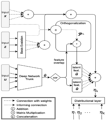
FIGURE 4.13: Architecture of SSDDR (X+Z (Struct.) and U (Unstruct.) Data) (Rügamer, Kolb, and Klein 2020).
If the mean is now modeled by both a linear and DNN part and the same feature inputs are fed to both model parts, we are in the setting of Wide & Deep NN. As illustrated above, such feature overlaps give rise to an identifiability issue. The key idea to mitigate this problem from Rügamer, Kolb, and Klein (2020) was to integrate an orthogonalization cell in the model, that orthogonalizes the latent features of the deep network part with respect to the coefficients of the linear and GAM part if feature overlaps are present. More precise, in case \(\boldsymbol{X}\) contains the inputs, that are part of the feature overlap, the projection matrix \(\boldsymbol{\mathcal{P}^{\perp}}\) projects into the respective orthogonal complement of the linear projection which is on the column space spanned by \(\boldsymbol{X}\). This allows backpropagation of the loss through the orthogonalization cell and therefore enables end-to-end learning. As the linear and GAM effect channels are directly connected to the distributional layer, the orthogonalization cell is therefore able to preserve the interpretability of the model.
Another way of orthogonalizing feature representations is by applying a two-stage procedure as described above. Law, Paige, and Russell (2019) utilize this procedure to make their latent feature representations retrieved from unstructured data orthogonal to their linear effect estimates from structured data. More specifically, they try to accurately predict house prices in London using multimodal DL on street and aerial view images as well as tabular housing attributes. Applying the two-stage procedure they aim at learning latent feature representations from the image data which only incorporate features that are orthogonal to the housing attributes. Thereby, they limit the chances of confounding in order to obtain interpretable housing attribute effects. Conducting a series of experiments, they find that including image data next to the tabular housing data does improve the prediction performance over single modality models albeit structured data remains the most relevant single data source. As a next step, they test their models with different model heads as depicted in the figure below to explore their respective potentials. Although fully nonlinear models with a DNN as model head generally offer larger modeling flexibility, as they can incorporate interactions, they achieved only slight performance gains over the semi-interpretable models with additive linear model heads. This is particularly interesting as the latter additionally preserve the often desired interpretability of effects. As the semi-interpretable models perform reasonably well, the authors argue that it is indeed possible to obtain interpretable models without losing too much on the performance side.
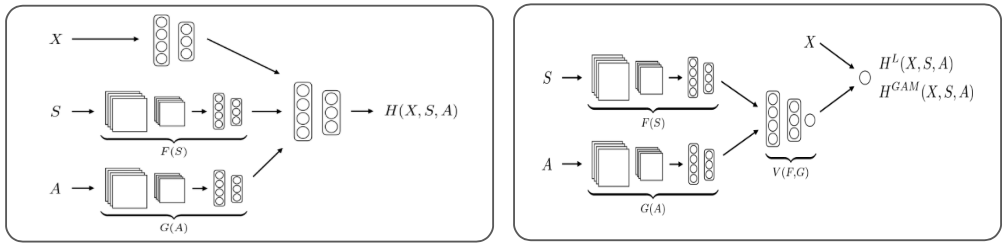
FIGURE 4.14: Fully Nonlinear and Semi-Interpretable Models (X (Struct.) and S+A (Unstruct.) Data) (Law, Paige, and Russell 2019).
In the last part of this section, we will allude to several other promising approaches that did pioneering work related to multimodal DL. While most of them use unstructured data sources such as remote sensing data, some do not specifically include structured data. They are still covered in this chapter to give the reader a broad overview of current research in the field. Moreover, structured data could easily be added to each of these models, but often studies intentionally avoid the use of structured data sources as they are sometimes scarcely available due to the cost of data collection. Besides availability, structured data such as household surveys is often irregularly collected and differs vastly between countries, making large scale studies impossible. Therefore, different studies have tried to provide alternatives to classical surveys by applying DL methods on freely available unstructured data sources. While Jean et al. (2016) use night and daylight satellite images to predict poverty in several African countries, Gebru et al. (2017) use Google Street View images to estimate socioeconomic attributes in the US. Both deploy the classical DL framework such as CNNs to retrieve relevant information from image data for the prediction task. Achieving reasonable prediction results while keeping analysis costs at low levels, both studies outline the potential of their proposed methods as being serious alternatives to current survey based analysis.
Other studies such as You et al. (2017) and Sirko et al. (2021) proposed DL frameworks for satellite imagery in contexts where labelled data is normally scarce. While You et al. (2017) use Deep Gaussian Processes to predict corn yield in the US, Sirko et al. (2021) apply CNNs to detect and map about 516 million buildings across multiple African countries (around 64% of the African continent). Besides being of great importance for applications such as commodity price predictions or financial aid distribution, the results of the two studies could easily be combined with other structured data sources and thereby could constitute a form of multimodal DL with high potential.
4.2.5 Conclusion and Outlook
In the previous sections we have come across various methods of multimodal DL that can deal with both structured and unstructured data. While these often differed substantially in their approach, all of them had in common that they tried to overcome limitations of classical modeling approaches. Examining several of them in detail, we have seen applications of different fusion strategies of data modalities and thereby touched upon related concepts such as end-to-end learning. The issue of interpretability was raised along several examples by discussing the advantages of different model heads as well as ways to solve identifiability problems using orthogonalization techniques.
It was indeed shown that it is possible to obtain interpretable models that are still capable of achieving high prediction performances. Another finding of past research was that end-to-end learning frequently showed to be superior compared to methods which learn feature representation via independent models or simply retrieve information via expert knowledge. Furthermore, research that actually conducted a comparison between their proposed multimodal DL and single modality models, almost always found their proposed multimodal model to outperform all models which were based on single modalities only. Nevertheless, within the class of single modality models, those using only structured data usually performed best. This leads to the conclusion that structured data often incorporates the most relevant information for most prediction tasks. By contrast, unstructured data sources may be able to add supplementary information and thereby partially improve performances.
While there certainly has been a lot of progress in the field of multimodal DL, conducted analyses still have their limitations which is why results need to be considered with care. Although most research finds their proposed multimodal DL models to achieve excellent performances, not all of them conduct benchmarking with regard to single modality models. Thereby, they limit the possibility to properly evaluate actual improvements over classical modeling approaches. Another aspect that may raise concerns regarding the reliability of results is that multimodal DL models such as most deep learning models have multiple hyperparameters. Together with the flexibility of choosing from a wide variety of data modalites, it opens up the possibility to tune the multimodal models in various ways. Thereby making it possible that actual performance improvements may only be existent for certain configurations of the model as well as combinations of data modalities. This problem is likely to be empathized for studies using only small datasets. Small datasets are especially common in the biomedical context where image data of certain diseases is normally scarce. On top of the previously mentioned aspects, publication bias may be a large problem in the field as multimodal DL models that do not show improvements over single modality or other existing benchmark models, are likely to not be published.
Although there might be concerns regarding the robustness and reliability of some results, past research has surely shown promising achievements that could be extended by future research. While small sample sizes especially for unstructured data such as clinical images were outlined as a great limitation of past research, more of such data will certainly become available in the future. As deep learning methods usually require large amounts of training data to uncover their full potential, the field will probably see further improvements once sufficiently large datasets are available. Hence, including only an increasing number of modalities with limited samples in the models will likely be insufficient. Instead, the most promising approach seems to be incorporating sufficiently large data amounts of certain unstructured and structured data modalities that contain relevant information for the problem at hand.
4.3 Multipurpose Models
Author: Philipp Koch
Supervisor: Rasmus Hvingelby
In this chapter, we will broaden the focus to include multitask learning additionally to multimodal learning. We will call this approach multipurpose models. Many multipurpose models have been introduced in recent years (Kaiser et al. (2017), Hu and Singh (2021b), Wang et al. (2022), Reed et al. (2022)), and the field gained attention. First, we will provide an in-depth overview of existing multipurpose models and compare them. In the second part, challenges in the field will also be discussed by reviewing the Pathways proposal (Dean 2021) and promising work addressing current issues for the progress of multipurpose models.
4.3.1 Prerequisites
At first, we will define the concept of multipurpose models and lay out the necessary prerequisites to make the later described models more accessible. We will introduce the definition of multipurpose models and further concepts that this book has not covered so far.
4.3.1.1 Multitask Learning
After the extensive overview of multimodal learning in the previous chapter, we now need to introduce multitask learning as another concept to define multipurpose models.
Multitask learning (Caruana (1997), Crawshaw (2020)) is a paradigm in machine learning in which models are trained on multiple tasks simultaneously. Tasks are the specific problems a model is trained to solve, like object recognition, machine translation, or image captioning. Usually, this happens using a single model, which does not leverage helpful knowledge gained from solving other tasks. It is assumed that different tasks include similar patterns that the model can exploit and use to solve other tasks more efficiently. The equivalent in human intelligence is the transfer of knowledge for new tasks since humans do not need to learn each task from scratch but recall previous knowledge that can be reused in the new situation. However, this assumption only sometimes holds since some tasks may require opposing resources, so performance decreases.
Multitask learning thus aims to achieve better generalization by teaching the model how to solve different tasks so that the model learns relationships that can be used further on. For a more in-depth overview of multitask learning, we refer to (Caruana 1997) and (Crawshaw 2020).
4.3.1.2 Mixture-of-Experts
Another prerequisite to this chapter is the mixture-of-expert (MoE) (Jacobs et al. (1991), Jordan and Jacobs (1994), Shazeer et al. (2017)) architecture, which is aimed at increasing the overall model size while still keeping inference time reasonably low. In an MoE, not all parts of the net are used but just a subset. The experts are best suited to deal with the input allowing the model to be sparse.
MoE is an ensemble of different neural networks inside the layer. MoEs allow for being more computationally efficient while still keeping or even improving performance. The neural networks are not used for every forward pass but only if the data is well suited to be dealt with by a specific expert. Training MoEs usually requires balancing the experts so that routing does not collapse into one or a few experts. An additional gating network decides which of the experts is called. Gating can be implemented so that only K experts are used, which reduces the computational costs for inference by allowing the model to be more sparse.
4.3.1.3 Evolutionary Algorithms
An evolutionary algorithm is used to optimize a problem over a discrete space where derivative-based algorithms cannot be applied to. The algorithm is based on a population (in the domain to be optimized) and a fitness function that can be used to evaluate how close a member of the population is to the optimum. Parts of the population are chosen to create offspring either by mutation or recombination. The resulting population is then evaluated with respect to their fitness function, and only the best-suited individuals are kept. The same procedure is repeated based on the resulting population until a specific criterion is met (e.g., convergence). While evolving the population, it is necessary to balance exploration and exploitation to find the desired outcome. Since EAs are research topics themselves and may vary heavily, we refer to (Bäck and Schwefel 1993) and, more recently, to (Doerr and Neumann 2021) for further insights.
4.3.1.4 Multipurpose Models
Now multipurpose models can be defined as multimodal-multitask models. Akin to the underlying assumptions of both learning paradigms, it can also be deduced that multipurpose models mimic human intelligence by marrying the concepts of multiple perceptions and transferring knowledge about different tasks for better generalization.
4.3.2 Overview of Mulitpurpose Models
In this section, we will closely examine existing multipurpose models. The main focus will be on how combining different modalities and tasks is achieved. At the end of this section, all models will be compared to provide a comprehensive overview of promising research directions.
4.3.2.1 MultiModel
The first prominent multipurpose model is the so-called MultiModel (Kaiser et al. 2017). This model, from the pre-transformer era, combines multiple architectural approaches from different fields to tackle both multimodal and multiple tasks. The model consists of four essential modules: The so-called modality nets, the encoder, the I/O Mixer, and the decoder.
Modality nets function as translators between real world data and a suitable representation for the inner modules. They also follow the purpose of back-translating, from the representation to the real world, to create output. For language tasks, the modality net is a tokenizer that outputs the appropriate embeddings, while for vision tasks, convolution operations transform the images into the proper representation. Furthermore, there are also nets for audio and categorical modalities. The modality nets embed the input into a unifying vector space which can be passed to the encoder. To produce the output, the representations from the decoder are fed into another modality net to produce the output. Language and categories are the only target modalities that have respective modality nets.
The core model consists of the encoder, the I/O mixer, and the decoder. Input is passed from the modality nets to the encoder first. Subsequently, the encoder passes its output further to the I/O mixer and the decoder. The decoder produces the output sequence. However, producing an autoregressive sequence requires knowledge of the previously generated sequence. Thus the output of the decoder is also read by the I/O mixer, which provides the decoder with the necessary information about the previous sequence. The I/O mixer passes its output back to the decoder to provide the necessary information. The decoder and I/O mixer require modality nets to read and write in the target modality. The encoder consists of multiple convolution operations and a mixture-of-expert layer. The I/O mixer and the decoder combine their dual input using cross-attention. A positional encoding conceptually similar to the one in transformers (Vaswani, Shazeer, Parmar, Uszkoreit, Jones, Gomez, Kaiser, et al. 2017b) is used for the attention mechanism.
MultiModel was trained on eight datasets, from which six were from the language modality and COCO (T.-Y. Lin, Maire, Belongie, Hays, Perona, Ramanan, Dollár, and Zitnick 2014b) and ImageNet (Russakovsky et al. 2015) from vision. For training, four experts in the MoE layers were used. The combined trained MultiModel on ImageNet and machine translation were below state-of-the-art (SOTA) models. Also, the combined model did not achieve significantly better results than a specialist model, which is the same model but trained solely on one task. However, it was found that the combined model did perform much better on a low-resource task than the respective specialist model.
MultiModel offers a pre-transformer approach to deal with different modalities on multiple tasks; although it is only used to generate text and clasification, the setup allows extending to other modalities easily.
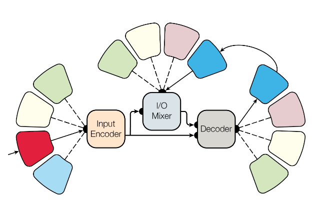
FIGURE 4.15: Architecture of MultiModel. The outer boxes without text are the modality nets. From Kaiser et al. (2017).
4.3.2.2 Unified Transformer (UniT)
A more recent multipurpose model is UniT (Unified Transformer) (Hu and Singh 2021b). UniT is built upon the transformer architecture, in which both encoder and decoder are used.
To account for multimodality and multitasking, the basic transformer (Vaswani, Shazeer, Parmar, Uszkoreit, Jones, Gomez, Kaiser, et al. 2017b) is enhanced. The encoder part of UniT consists of two modality-specific encoders since the initial setup is aimed at the modalities of text and vision. However, more modality-specific encoders may be added. For the case of language, a BERT model (Devlin et al. 2018b) is used, while a detection transformer (DETR) (Carion et al. 2020) encoder is used for vision. DETR uses a particular approach to feed images to the encoder. At first a CNN is used to create a lower dimensional representation of the input image, which is then reorganized as a sequence. This sequence is then fed into the encoder following Vaswani, Shazeer, Parmar, Uszkoreit, Jones, Gomez, Kaiser, et al. (2017b). The [CLS] token is also used in the BERT encoder, which is also included in the output sequence of the encoder. A task-specific token is additionally added to the input of the encoders. The output of the encoders is then concatenated to form a single sequence. The decoder is fed with this sequence and a task-specific query. Since the decoder architecture sticks to the DETR model, the decoder does not produce a sequence autoregressively. Instead of taking the previously produced sequence (autoregressively) as input, the decoder is fed with the task-specific query vectors instead, thus producing a uniform output. On top of the decoder are task-specific heads needed to transform the decoder output into the desired shape for the specific task.
For training, the object detection task requires bounding box loss from DETR, while the other tasks use cross-entropy loss.
In experiments, UniT was evaluated against a single-task version of itself. The general model outperformed the specialist one on multimodal tasks but was outperformed on unimodal tasks by the specialist UniT. UniT was furthermore also outperformed by SOTA models, although the numbers remained comparable.
Even though UniT does not achieve SOTA or consistently outperforms its specialist version, it is a powerful method to achieve a simple multipurpose model. By using available encoder models, it is easily extendable.
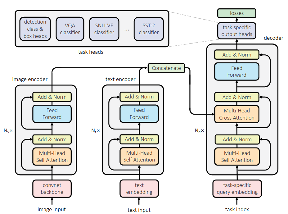
4.3.2.3 OFA - Sequentialization is All You Need
Another multipurpose transformer is OFA (Once For All) (Wang et al. 2022). To utilize the sequence-to-sequence (seq2seq) architecture of the transformer, all input is transformed into a seq2seq problem.
While MultiModel and UniT use specific modules for a modality (modality nets and modality-specific encoders), a different approach is used for OFA. All input is sequentialized and embedded in a shared representation space. Since tokenizing an image using a vocabulary is not feasible, a similar approach to ViT (Dosovitskiy, Beyer, Kolesnikov, Weissenborn, Zhai, Unterthiner, Dehghani, Minderer, Heigold, Gelly, and others 2020) is used (where input is flattened to 16 x 16) to obtain a sequence of \(P\) representations. These representations are in the same dimension as the token embeddings from text input, which are tokenized using Byte-Pair-Encoding (Sennrich, Haddow, and Birch 2016). After feeding the embeddings through the encoder, the decoder produces the output as a sequence again. However, in this case, images are represented as a sequence of tokens, similar to the image-patch vocabulary in DALL-E (Ramesh, Pavlov, et al. 2021d). Furthermore, a special sequence for bounding boxes is also used for object detection and recognition. To generate the task-specific solution, it is thus required that another model is used to generate the images based on the tokens and to visualize the bounding boxes based on the obtained coordinates.
Since OFA is an autoregressive model (the probability for the next token is predicted based on the previously produced tokens and the input provided), the objective is based on cross-entropy loss. OFA was trained on different crossmodal tasks: visual grounding, grounded captioning, image-text matching, image captioning, and visual question answering. Further unimodal tasks for training did include: image infilling, object detection, and text reconstruction as in BART (Lewis et al. 2020).
OFA outperformed SOTA models on cross-modal tasks like image captioning, visual question answering, visual entailment, and visual grounding. On uni-modal tasks, OFA performed well, although it did not outperform SOTA models. OFA showed additional transfer capabilities to unseen tasks, which were presented with an additional description to solve the task in a few-shot manner. Although the results were satisfactory, the model was not evaluated against a specialist baseline.
OFA proved to be a powerful model that is capable of using the entire transformer architecture by sequentializing all input and thus producing tokenized output.
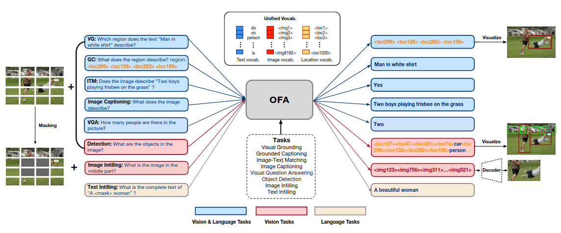
FIGURE 4.17: OFA, the different input and output concepts can be seen here. From Wang et al. (2022).
4.3.2.4 Gato - A Generalist Decoder
Another model that utilizes the seq2seq approach in transformers is Gato (Reed et al. 2022). The model can be used as a language model, an agent to play games, and an agent to control robotics.
As in OFA, problems are transformed into a seq2seq problem, on which a transformer (decoder only) is applied. Every input from text, vision, robotics, and games is represented sequentially. Visual input is encoded using a flattened sequence of 16x16 patches fed into a ResNet (He et al. 2015), while text input is tokenized using SentencePiece (Kudo and Richardson 2018). Furthermore, discrete values like buttons in games and continuous data like movements from robotics are tokenized in a vocabulary too. To represent all modalities sequentially, the different tokens are concatenated. A separator token “|” is added to distinguish the observations from the following action, so that a sequence looks simplified as the following:
\[\left [ ... \left [ x_{\textrm{Text}}, x_{\textrm{Images}}, x_{\textrm{Discrete and Continuous Values}}, |, y_{\textrm{Action}} \right ]_i, ... \right ]\]
By using this approach, the transformer can predict the next action autoregressively since it is a sequential problem. In the case of text, the action token is also a text token. Since it is only necessary to predict the action based on the previous values, a mask function is added to the cross-entropy loss function, which masks the previous values so that only the next action is predicted and not the conditions for the action. The masking function is always one for text since every previous text token is necessary for language modeling.
Gato was evaluated on reinforcement-learning-based (RL) tasks against specialist RL agents, where Gato performed worse than the specialist agents. On unseen tasks, Gato required fine-tuning since few-shot learning is not feasible due to the input length restrictions in transformers. However, the results were mixed. Some improvements were possible, and the expert was outperformed, but in other cases, massive fine-tuning efforts only led to small gains. It was found that the generalist agent outperformed the specialist agent (particularly trained for this task) most of the time. Only at the specific Atari Boxing (Bellemare et al. 2013) task, Gato was outperformed by the specialist Gato model. Both performed much lower than another task-specific model used as a baseline. In robotics, Gato showed comparable behavior to the baseline SOTA model. Additionally, Gato also showed capabilities in image captioning and dialogue modeling, although these aspects were not elaborated further.
Like OFA, Gato can sequentialize all input and produce a sequential output that can be back-transformed to solve a task. It was shown that Gato could sometimes transfer knowledge on unseen tasks and outperform the specialist agent most of the time.
4.3.2.5 Comparison
Although many tasks and modalities lead to a curse of dimensionality for comparison, the architectures and the respective modifications of the introduced systems remain simple to compare.
A trend toward seq2seq models can be seen with MultiModel, OFA, and Gato solving tasks in a seq2seq manner. The most prominent similarity is the transformer architecture used entirely (encoder & decoder) in OFA and truncated (decoder only) in Gato. Another significant similarity between both architectures is the use of a particular ordering of input and output. In Gato, the sequence is organized around predicting an action using a special token, while OFA produces a sequence as a solution which can be the bounding box or the sequence of an image to be fed in the generator module. While Gato can solve tasks from robotics and game playing, OFA can also generate images. However, both architectures require specific modules to decode the tokens into the respective modality.
Gato and OFA both use a shared representation space. Minor details differ, so the image tokenization process is different, and additionally, Gato can encode more modalities than the published version of OFA (although extending OFA is theoretically simple).
MultiModel also show some familiar characteristics. The architecture is from the pre-transformer age but also brings many characteristics of the transformer architecture, like the use of attention, positional encodings, and encoder-decoder. Since the output in the presented version only produced text or classification separately, there is no need for special orderings used in OFA and Gato. The necessity to produce the modality-specific output in modality nets is similar to the generator module in OFA that produces images. However, the tokens are already produced in an intermediate step in OFA, while the modality nets are crucial to producing the final output in MultiModel. UniT follows an entirely different approach that is more pragmatic by leveraging the contextual capabilities of the transformer decoder. M modalities can be encoded as a sequence on which the transformer decoder fuses the modalities and learns the relationships. The use of special tokens for each task and task-specific heads, focus the model on the requested task yet also requires tuning the model specifically.
None of the models besides OFA achieved SOTA results. Compared to specialist models, the general models were comparable in their results (Gato, UniT, MultiModel). MultiModel, OFA, and Gato showed transferability on low-resource or unseen tasks. However, more research in this direction is highly recommended. MultiModel was only compared on a low-resource task against a specialist model, and OFA was not compared to another model for the unseen task. Gato performed better than a specialist model, trained from scratch on most unseen tasks, but failed against the untrained specialist model in Atari Boxing.
| Model | Approach | Modalities | Outperformed Specialist Model? | Unseen Tasks? | Number of Parameters | Year |
|---|---|---|---|---|---|---|
| OFA | Seq2Seq | Vision, Text | Yes | 33M-930M | 2022 | |
| Gato | Seq2Seq | Vision, Text, Robotics, Discrete Entities (e.g., Buttons) | In most cases | Yes | 79M-1.18B | 2022 |
| UniT | m Encoders, task-specific head | Vision, Text | No | No | 201M | 2021 |
| MultiModel | Different modality nets for Seq2Seq | Vision, Text, Audio, Categorical | Comparable | Excelled on low resource task | Unknown | 2017 |
Comparing the models among each other becomes difficult with more modalities and tasks, which is its own curse of dimensionality. For example, Gato also included robotics and RL, which none of the other models included. MultiModel also has a modality net for sound, while UniT and OFA only worked for vision and text. Further research into the comparability of multipurpose models becomes essential.
4.3.3 Pathways and Promising Works
Although models have become more capable of solving complex tasks, significant limitations remain. A persisting issue in current deep learning is the necessity to train from scratch and disregard already obtained knowledge, which is highly ineffective compared to human intelligence. Another issue arises from the evergrowing, dense networks that requires more and more resources.
In this section, we will review the Pathways proposal (Dean 2021) and promising techniques to address these issues. Overcoming these problems would be especially beneficial for multipurpose models. Reusability of knowledge is crucial for the multitask perspective, and improving the performance of potentially billion-parameter-sized models will also have a significant positive impact.
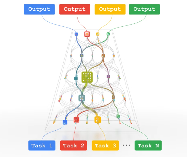
FIGURE 4.18: Concept of Pathways. Different tasks follow different paths to different expert models. From Dean (2021), Screenshot August 31th 2022.
4.3.3.1 Pathways Proposal
Pathways (Dean 2021) follows a different idea than previously seen methods. The model consists of a large graph through which data can be forward passed. The nodes of the network are neural networks themselves. A pass through this network does not include passing all nodes and thus not all neural networks, but only a few. The pass follows a specific path from one entry to the network’s exit. The underlying idea behind this is similar to the mixture-of-expert models described previously. Only the specific networks dedicated to solving a problem are to be activated during inference.
At this point, it is necessary to recall that multitask learning aims to generalize better on new tasks since the knowledge about previously learned tasks can be applied. This idea is the foundation of Pathways too, where specialist networks (nodes) are combined in a larger network. It is assumed that the model’s generalization capabilities increase significantly by finding an appropriate path for a task to the appropriate expert nodes. In this setup, the particular task-specific problem-solving capabilities are combined. Furthermore, multimodality is also considered as a potential extension. Adding more modalities might not be a difficult problem considering the architecture of the previously introduced transformer-based models. Overall the approach of a sparse model combining multiple experts offers many opportunities to combine modalities and reuse task-specific capabilities. The sparsity of the model offers decreased inference time since only few parts of the networks are activated during inference.
Another aspect of the Pathways proposal includes the improvement of current hardware limitations. It is already observable that Moore’s Law (each n years, the compute capacity doubles) has been slowing down substantially, while deep learning research has grown exponentially in the late 2010s (Dean 2020). Thus, hardware also needs to be adapted to the growing demand in deep learning. In the context of the pathway proposal, a novel framework for Google data centers has been introduced, aiming to reduce overhead during computation and access specific parts of the model to utilize the technical advantages of sparse networks. As opposed to dense models where a whole model must be accessed, with sparse networks it is not necessary to use the whole network but only chunks of it. So far, two large pre-trained models have been introduced based on the new training framework. One is the Pathways Language Model (PaLM) [Chowdhery2022], which is currently the largest language model using 540 billion parameters, Minerva (Lewkowycz et al. 2022). Minerva is based on PaLM, and Parti (J. Yu, Xu, Koh, et al. 2022a),
4.3.3.2 PathNet
An earlier approach for a sparse multitask network, which looks deceptively similar, is PathNet (Fernando et al. 2017). PathNet is a training concept that reuses knowledge from a previously learned task without the risk of catastrophic forgetting (knowledge is overwritten), thus using solely the positive aspects of multitask learning. The objective of PathNet consists of a evolutionary algorithm (EA).
Neural networks are often depicted as a graph in which the input is directed to all nodes in hidden layers, and their output is again passed to all nodes in the next hidden layer or an output layer. In the case of PathNet, each node is itself a neural network. The training algorithm finds the best paths for a specific task through the network.
At first random paths through the network are initialized, then the paths are trained for T epochs. After training, the paths are evaluated against each other. The winning path overwrites the losing path. However, to achieve exploration, the overwritten path is mutated by randomly including neighbors of the winning path. Until a specific criterion to stop (e.g., number of epochs) is reached, the current paths are frozen so that no more modifications to the parameters of the networks on this path are possible. All other parameters are newly initialized again. Also, a different, task-specific head is initialized. The same procedure is now done again for the next task. Then, the main difference is that the previously obtained path, including the trained networks, is frozen during training so that the model can transfer knowledge from the previous task to the new task. The model then finds appropriate paths throughout the network until the stopping criterion is met again.
PathNet was evaluated on supervised learning tasks and RL scenarios. Learning from scratch and fine-tuning a PathNet, were chosen as a baseline. For fine-tuning, the first path was chosen as a base model that was fine-tuned on the second task. Overall, PathNet improved training time and prediction quality for the second task compared to standard fine-tuning and learning from scratch. PathNet has shown that different tasks can reuse the knowledge from training on previous tasks without suffering from catastrophic forgetting.
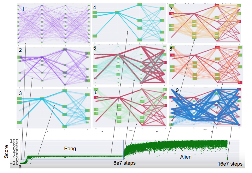
FIGURE 4.19: (ref:pathnet)
(ref:pathnet) Training PathNet on two tasks. At first random paths are initialized (1), then trained (2-3) and fixed (4). The same procedure is repeated for the next paths using the previously fixed paths and new parameters in all other nodes (5-9). From Fernando et al. (2017).
4.3.3.3 LIMoE
LIMoE (Multimodal Contrastive Learning with LIMoE: the Language-Image Mixture of Experts) (Mustafa et al. 2022) combines text and vision input using a MoE-enhanced transformer encoder.
While previous methods used two models (two-tower) to encode modalities, LIMoE is solely based on one model, where the modalities are processed in a single modified transformer-model (one-tower). The text data is encoded using One-Hot-SentencePiece (Kudo and Richardson 2018) encoding, while images are tokenized in the same way as in ViT (Dosovitskiy, Beyer, Kolesnikov, Weissenborn, Zhai, Unterthiner, Dehghani, Minderer, Heigold, Gelly, and others 2020) (elaborated further in the previous chapter) to provide the input appropriately. The main difference to the standard transformer is an MoE layer where the feed-forward network usually lies. In this layer, E experts are used, which are themselves feed-forward-networks. For each token,K appropriate experts will map the tokens further downstream. The routing is computed by a gating net network, which decides which K experts are called. Another feature here is a fixed-length buffer for each expert in the MoE layer. This buffer is used to store tokens before an expert network processes them, assuming that the allocations of tokens for each expert are balanced. If it is impossible to buffer tokens for the experts, the tokens will be dropped. To process the more important tokens first, Batch Priority Routing (Riquelme et al. 2021) is used to provide a ranking mechanism. The output of the transformer encoder is then average pooled and subsequently multiplied with a modality-specific weight matrix, which produces the eventual output for the token of both modalities.
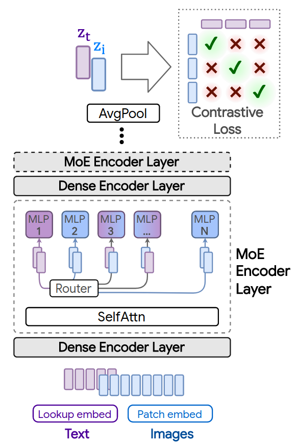
FIGURE 4.20: Architecture of LIMoE. From Mustafa et al. (2022).
The model is trained using a contrastive objective. In this case, the contrastive loss aims to maximize the paired visual and textual input while minimizing all combinations of unpaired embeddings. This objective can be achieved by using the dot-product as a similarity measure between the embeddings of both modalities, which provide a differentiable operation through which the overall loss can be minimized.
Additionally, the pitfalls of a multimodal MoE are also considered. One challenge in MoE is the correct balancing of routing to the experts, which is even more challenging when using unbalanced multimodal data. To address this issue, two new losses based on entropy are introduced. Entropy can be used as an appropriate term since it provides a valuable number for the uniformity of the distribution, which is necessary to balance the expert assignments. The losses are aimed at controlling the allocation of experts to tokens, which is also necessary to fulfill the assumptions for the implemented buffer. One loss considers the token level (local) routing distribution, and the other considers the overall expert routing distribution (global). The local loss aims to achieve no uniform behavior in expert allocation such that each token is indeed assigned to specific experts. In contrast, the overall global loss aims to achieve uniformity over all tokens to avoid a collapse in which tokens are solely assigned to a few experts which do not have the capacity to deal with all tokens. These losses are computed for each modality. Furthermore, already available losses for training MoE models were also added to avoid known downsides of MoE models.
LIMoE was compared against similar models like CLIP (Radford, Kim, Hallacy, Ramesh, Goh, Agarwal, Sastry, Askell, Mishkin, Clark, and others 2021). The test dataset was ImageNet (Deng et al. 2009) and COCO (T.-Y. Lin, Maire, Belongie, Hays, Perona, Ramanan, Dollár, and Zitnick 2014b). Overall, LIMoE-H/14 (largest model, 12 MoE-layers, 32 experts per layer) achieved strong performance considering that only one model was used for two modalities against specialist models in two-tower setups. It was also possible to outperform CLIP by a significant margin while using minimal additional parameters. Models that achieved similar results to LIMoE used at least twice the number of parameters for a forward pass.
LIMoE provides an example that an MoE-based model achieves impressive results in a multimodal model. Current language and vision encoding techniques are combined and married with the upsides of the MoE-architecture, leading to a single model that can outperform current state-of-the-art models like CLIP.
4.3.3.4 muNet (Multitask Network)
muNet (Gesmundo and Dean 2022) is an architecture that maximizes the reusability of previously learned knowledge by using an evoluationary algorithm to evolve a new model. The authors address the current practice for fine-tuning, where a pre-trained model is copied and then explicitly trained on a task by overwriting previous knowledge.
An initial model is evolved by using an evoluationary algorithm to fit specific tasks, while keeping the previously learned knowledge. Eventually, a set of models is obtained, which includes new neural networks, based majorly on the parameters of the initial model. The new modules can be seen as paths to task-specific modifications of the initial network.
The EA of muNet starts with an initially proposed model that is mutated further on. All further mutations are stored so that after a set of candidates is available, the set can be split into models trained for this task (active population) and models for other tasks (inactive population). These two sets become the sets of candidates for the following task-specific iterations. Training a specific task follows three steps: Sampling candidate models, mutating, training, and evaluation. The best scoring model is added to the active population for further mutation. A sampling algorithm accounts for exploration and exploitation to get a candidate model for subsequent mutation. The active population is ordered in a descending list based on the model’s score. Each list entry is then revisited, starting from the highest scoring model onward, so that the better performing models are considered first (exploitation). The draw probability is computed as:
\[\mathbb P(m|t) = 0.5 ^{ \#timesSelected(m, t)}\]
Where \(\#timesSelected(m, t)\) is the amount of previous mutations based on model m for task t). The more unsuccessful mutations the model has had before, the smaller the draw probability becomes. Thus, exploration is emphasized by considering previous attempts and allowing other models to be preferred as well. However, if this method does not yield a candidate, a model is drawn from the union of the inactive and active population. Applying mutations is the next step in the algorithm. A random number of mutations are drawn from the set of possible mutations, which include:
- Layer Cloning: A layer is cloned for training. The layer’s parameters are copied from the parent model so that training can continue using the same knowledge. The other layers are still used but are not updated. Additionally, the task-specific head layer is cloned to account for the underlying changes. In case of training on a new task, the head is also newly initialized.
- Layer Insertion: Two layers are added to the model as residual adapters ((Rebuffi, Bilen, and Vedaldi 2017), [Houlsby2019@]). The second layer is zero-initialized to keep an identity function so that training can continue from the state before mutation.
- Layer Removal is used to skip layers while still using all other layers of the parent model in a frozen state.
- Hyperparameter Change: samples hyperparameters close to the ones of the parent model. A list of neighboring values is constructed from which a parameter is drawn.
Subsequently, the models are trained on the task and scored. If the mutated model is better than the parent model, it is also added to the task’s set of active models. This routine is done for all tasks iteratively and can be repeated several times. Ultimately, only the best scoring models are kept for each task, yielding a list of models each fit to a particular task. muNet was evaluated for fine-tuning against a ViT instance, which was aimed at being the most generalizable one (Steiner et al. 2021). The evaluation benchmarks consisted of multiple classification problems (to simulate multitasking). ViT was fine-tuned on all of these tasks as a baseline. In contrast, another ViT was evolved using muNet, on which the baseline model was evaluated again. The approach using muNet outperformed the fine-tuned ViT while using significantly fewer parameters.
muNet offers a simple, evolutionary-based approach for fine-tuning and keeping all previously acquired knowledge safe, thus maximizing reusability.
4.3.4 Conclusion Pathways
The introduced models show promising novel features that might improve multipurpose models. However, these models can only be improved if research is done to combine the distinct concepts. PathNet and muNet offer novel approaches to leverage already acquired knowledge, while LIMoE improves handling different modalities in a single, sparse model. Furthermore, it also becomes necessary to conduct research into scaling these concepts up. Since the multitask-related models (PathNet and muNet) only included a few tasks, introducing more tasks for training and testing might offer insights into how transfer between tasks succeeds and fails.
LIMoE offers a promising architecture with respect to performance. Due to the sparsity of the MoE-layer, LIMoE is faster, while it also outperforms previous dense models. Using MoE-layers in transformers might also be a viable path for models like OFA and Gato. Combining the flexible encoding techniques of these models with the relative sparsity of LIMoE might result in even more capable and efficient models. We, therefore, recommend further research in this direction.
Another potential path for future research is intelligent routing for evolving methods like muNet and PathNet. Evolutionary models offer a promising approach to leveraging previous knowledge. However, the resulting models are tailored to a particular task. Novel routing techniques to send data to dedicated expert nodes in a complex network of models might help models generalize, as was outlined in the Pathways proposal.
4.3.5 Discussion
We reviewed multipurpose models that have become capable of solving multiple tasks from different modalities. The transformer architecture also boosted the development in this field, in which three of the four presented models were transformer-based and from recent years. Multipurpose models offers an opportunity to use one model instead of many different expert-models. Furthermore, some multipurpose models (Gato, OFA) also outperformed expert-models. However, Gato also showed inferior performance on ATARI Boxing compared to competing models, indicating that research is still required to explore the relationship between tasks. We also presented promising novel architectures that alleviate or may solve problems in current multipurpose models. However, further issues remain that have not been solved by research to this day:
A pitfall of models of these sizes is the low accessibility. Researchers need to access the model through an API since running these models on a few GPUs will likely be infeasible. It might be unlikely to see a BERT-like engagement with the community of researchers if the access to models remains limited. On the contrary, more open-source collaborations, as seen with EleutherAI or Huggingface, might evolve as well as a countermovement and techniques like distillation (Hinton, Vinyals, and Dean 2015) might become more critical.
Another issue with multipurpose models is the lack of metrics. Current metrics are not suited for multitask and multimodal models. Evaluation might also become harder since many different modalities can be used, as seen here with the robotics property of Gato, which was not used in any of the other reviewed models.
Eventually, it is also necessary to consider the societal impact. The bias problem will also become an issue in multipurpose models, especially since multiple datasets must be considered.
Also, the environmental impact of training large models needs to be considered since it is likely that larger models will yield better performance according to scaling laws (Reed et al. 2022) but will also have a larger carbon footprint.
4.4 Generative Art
Author: Nadja Sauter
Supervisor: Jann Goschenhofer
FIGURE 4.21: LMU logo in style of Van Gogh’s Sunflower painting
As we have seen in subsection 3.2, computers can create images only based on text prompts via multimodal deep learning. This capability is also used in digital arts in the field of ‘generative art’ or also known as ‘computer art’. The new movement comprises all artwork where the human artist cedes control to an autonomous system (Galanter 2016). In this way everyone, even artistically untrained people, can easily create pictures as the computer takes over the image generation. In some way, the computer becomes the artist with some sort of creativity, a distinct human ability. In this chapter, we want to give an overview about how computers improved over time in generating images and how this is used in the contemporary arts scene. For instance in Figure 4.21 we used the seal of the Ludwig Maximilians University and changed the style to Van Gogh’s Sunflower painting by the Neural Stlye Transfer Algorithm and the method CLIP + VQGAN which fuses the logo with sunflowers in a Van-Gogh-style way.
4.4.1 Historical Overview
The first attempt to use AI to generate pictures was made by the engineer Alexander Mordvintsev (2015) and his “DeepDream” Software. He used Convolution Neural Networks to generate very interesting and abstract images based on the activation of a layer, visualizing the patterns learned by a neural network. Below you can see a picture of a Labrador after it was processed by the DeepDream algorithm.
FIGURE 4.22: Picture of a Labrador processed by DeepDream (Google Colab)
In the following year, Gatys, Ecker, and Bethge (2016) investigated methods to transfer the style of pictures. This method was used to transfer the style of Van Gogh’s Sunflower painting to the LMU seal at the beginning of this chapter (see Figure 4.21). Besides, below in Figure 4.23 you can see the same Labrador picture from Figure 4.22 in Kandinsky style.
FIGURE 4.23: Picture of a Labrador with Kandinsky style (Google Colab)
Furthermore, the architecture of Generative Adversarial Networks (GANs), which was first introduced by I. Goodfellow et al. (2014), was used by another research group Karras, Laine, and Aila (2019) to create very realistic fake images with their architecture StyleGAN. For instance, one can create pictures of people who do not exist, but look totally realistic (see Figure 4.24).
FIGURE 4.24: Fake face generated by StyleGAN
Nevertheless, it was almost impossible to control the exact output of these early forms of AI art. There was no option to make specifications of how the result should look like in detail. For instance, you always get a human face with the earlier mentioned StyleGAN application, but you cannot specify to generate a blond girl with green eyes. This can be achieved by applying the artist-critic paradigm (Soderlund and Blair 2018): Thereby, the computer as an artist generates a picture based on what the Neural Network learned in the training phase (e.g. StyleGAN learns to generate pictures of human faces). Additionally, a critic is used to tell the computer if the output satisfies the concrete idea of the human artist. For this reason multimodal deep learning models emerged in the field of generative art. Here, one can control the output with the help of text prompting. In this way one can check if the generated picture matches the initial text description. Looking at the previous StyleGAN example, the multimodal architecture supervises whether the output picture is indeed a blond girl with green eyes or not. A new class of models for generating pictures evolved.
This idea was used by OpenAI for their models DALL-E (Ramesh, Pavlov, et al. 2021a) and CLIP (Radford, Kim, Hallacy, Ramesh, Goh, Agarwal, Sastry, Askell, Mishkin, Clark, Krueger, et al. 2021a) which were released in January 2021. Both architectures are critics for multimodal models. Only a few days after the release, Ryan Murdock combined CLIP (critic) with the already existing Neural Net “BigGAN” (artist) in his “The Big Sleep” software. Furthermore, Patashnik et al. (2021) developed StyleCLIP, a combination of StyleGAN (artist) and CLIP (critic) to edit parts of images via text instructions. In the following months, Katherine Crowson combined CLIP as critic with the existing VQGAN algorithm as an artist. She also hooked up CLIP with guided diffusion models as artists to yield more fine-grained results. This approach was further investigated by OpenAI that published a paper (Dhariwal and Nichol 2021) in May 2021 about guided diffusion models. Moreover, in December 2021 they introduced GLIDE (Nichol et al. 2021a), a model with CLIP or classifier-free guidance as critics and diffusion models as artists. For more technical details about text2img methods like DALL-E and GLIDE refer to subsection 3.2 or for text supporting CV models like CLIP at subsection 3.4.
4.4.2 How to use these models?
A lot of different notebooks are publicly available to apply the different pre-trained models. In general, all notebooks work pretty similar: one only needs to enter a text prompt in the code and after running the notebook the computer generates a picture based on these instructions. It is relatively easy and no prior coding knowledge is required. Moreover, there are also some API and GUI applications (e.g. MindsEye beta) where no programming knowledge is needed at all. Using these models, it is important to think about how exactly once enters the respective text prompt. One can influence the output in a desired way with little changes in the short text instruction. This is also known as “prompt engineering”. For instance, in the beginning of this chapter, we entered the prompt “in the style of Van Gogh” to change the style of the LMU seal. In this context, a special trick is to append “unreal engine” (Aran 2021) which makes the resulting pictures more realistic with higher quality. This seems surprising at first, but the models were trained on data from the internet including pictures of the software company Epic Games that has a popular 3D video game engine called “Unreal Engine”. This is one of the most popular prompting tricks.
Unfortunately, OpenAI has never released DALL-E. There is only an open-source version called ruDALL-E (Shonenkov 2021) that was trained on Russian language data. Besides, hugging face hosts DALL-E mini (Boris 2022) where one can generate pictures, but does not have access to the model itself. PyTorch offers a replication of the DALL-E code (OpenAI 2021) but no trained model. Furthermore, CLIP was released without publishing the used training data. However, there exists an open source data set with CLIP embeddings called LAION-400m (Christoph Schuhmann et al. 2021b). In the following, we used different publicly available notebooks to try out the different models CLIP + BigGAN, CLIP + VQGAN, CLIP + Guided Diffusion, GLIDE with the text prompt “a fall landscape with a small cottage next to a lake” (see Figure 4.25) and “panda mad scientist mixing sparkling chemicals, artstation” (see Figure 4.26). The first prompt shows pretty realistic results, whereas the second prompt results in more different and “crazy” outputs. That is because the panda-prompt is more abstract than the first one and hence more difficult to illustrate. In addition, some of the notebooks run on lower resolution due to computational limitations. Besides, GLIDE is also downsized by the publisher: The released smaller model consists of 300 million parameters, whereas the unreleased model has about 3.5 billion parameters (Nichol et al. 2021a). So better results are possible with higher computational power and other implementations of the models.
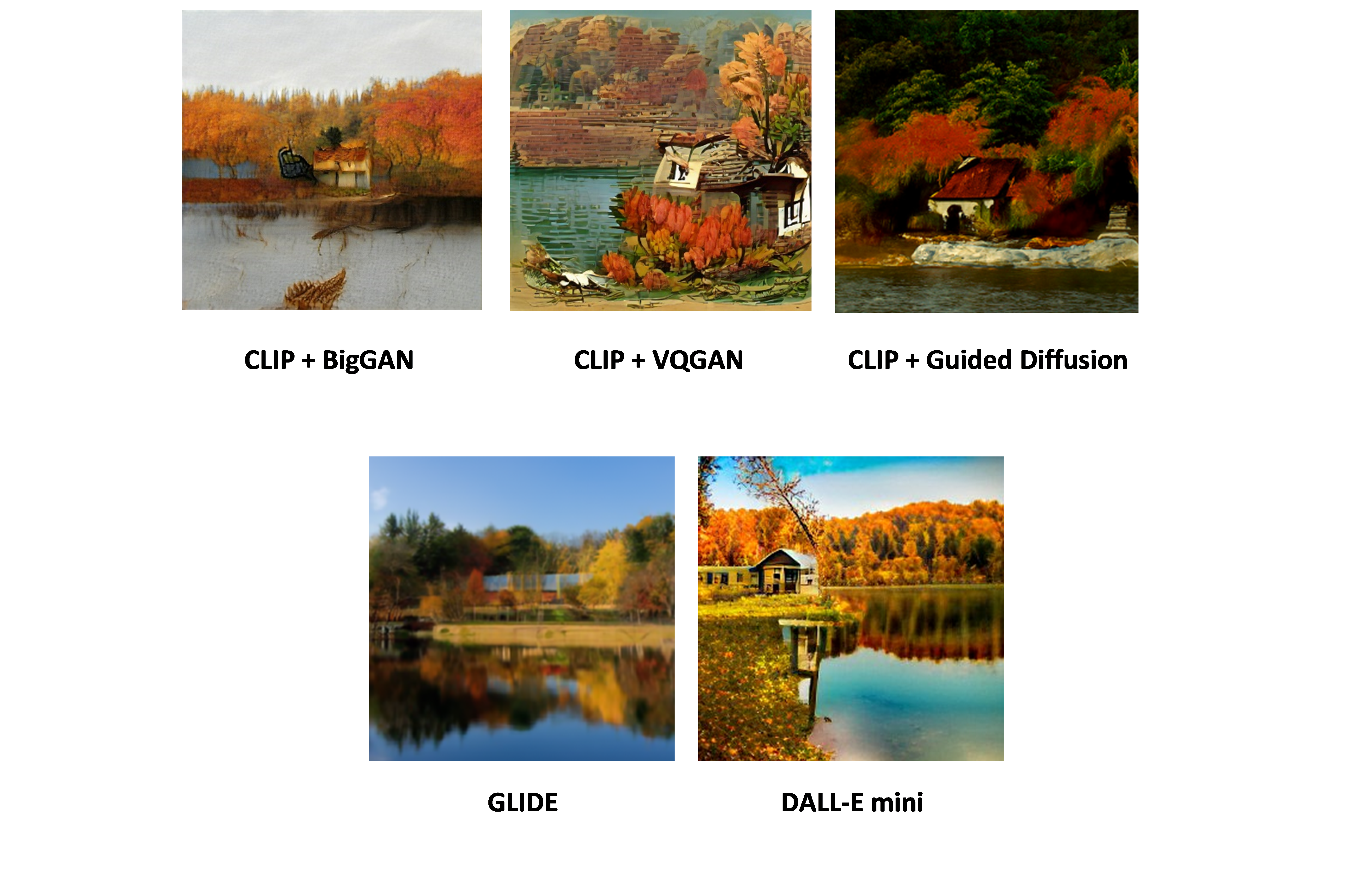
FIGURE 4.25: Comparison of different models with prompt “fall landscape with a small cottage next to a lake”
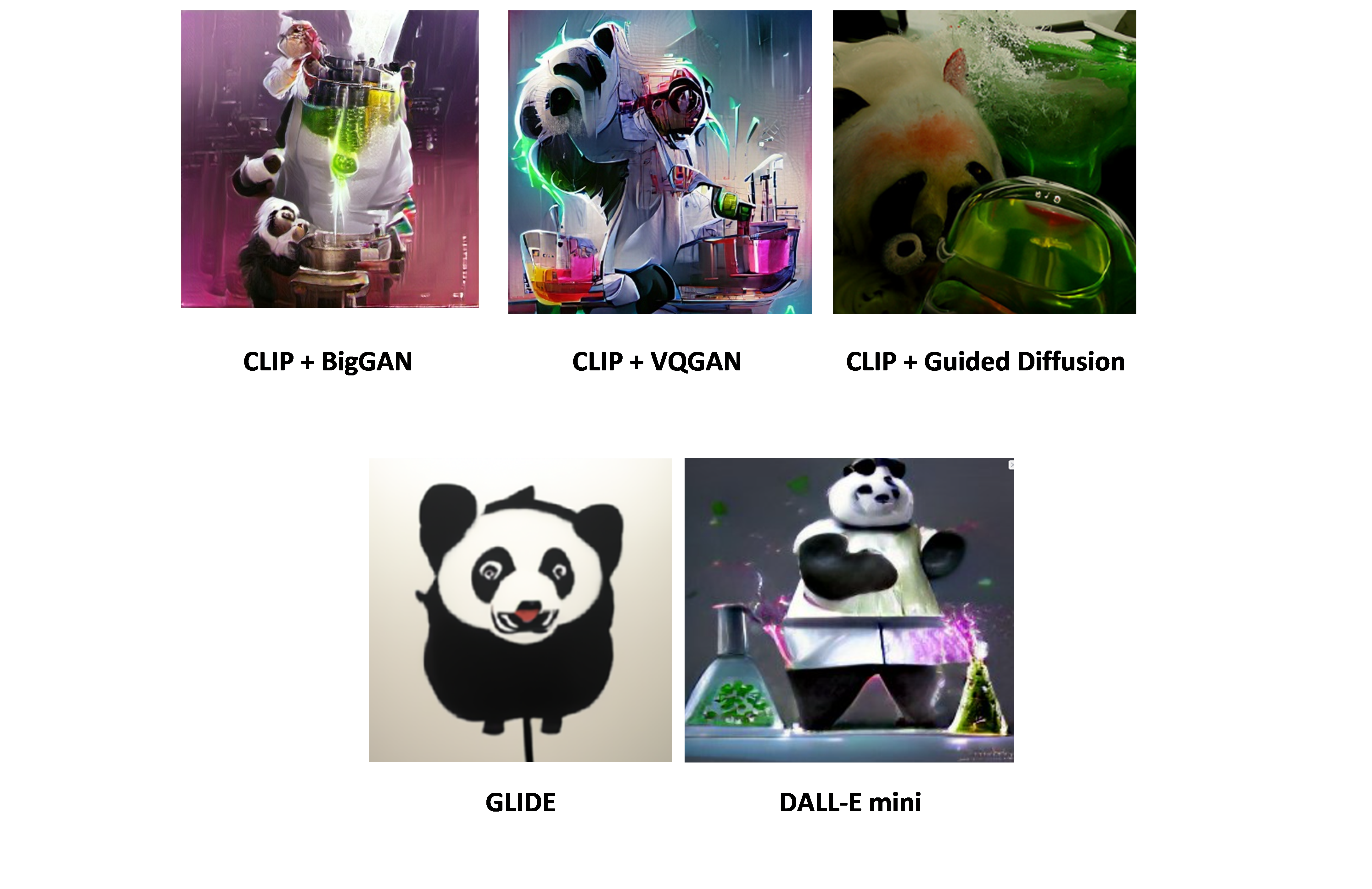
FIGURE 4.26: Comparison of different models with prompt “panda mad scientist mixing sparkling chemicals, artstation”
4.4.3 Different tasks and modalities
So far, we concentrated on the two modalities text and image. Combining both of them, one can tackle different tasks with the models mentioned above. The main usage is to generate images based on a text prompt. Therefore, one can start from noise or but is also possible to chose a real image as starting point (Qiao, Liu, and Chilton 2022). This was done in the beginning with the LMU seal by CLIP + VQGAN (see Figure 4.21): instead of starting from noise, the model started from the LMU seal as initialization and then used the prompt “in style of Van Gogh”. The video captures how the model develops during fitting. In the end, the typical Van Gogh sunflowers emerge as well as what could be a part of Van Gogh’s face.
Furthermore, one can edit, extend, crop and search images with models like GLIDE (Nichol et al. 2021a). For instance, Nichol et al. (2021a) fine-tuend the model for text-conditional image inpainting (see figure 4.27). By marking some area in the pictures, here in green, and adding a text prompt, one can edit pictures very easily and precisely. This is quite impressive as the model needs to understand from the text prompt which object should be filled in and then do this in the correct style of the surrounding to produce a realistic outcome. Another idea is to use a sketch of a drawing and let the model fill in the details based on a text caption (see figure 4.28 below). This allows controlled changes of parts of pictures with relatively little effort. In this way, GLIDE can be used to generate pictures out of random noise, but also to edit pictures in a specific way. Furthermore, it is also possible to combine other modalities as well (see more details in subsection 4.1). For instance, WZRD (2020) accompanies custom videos with suitable audio. It is even imaginable to create sculptures with 3D-printers (Mccormack and Gambardella 2022).
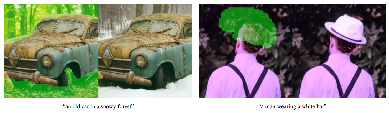
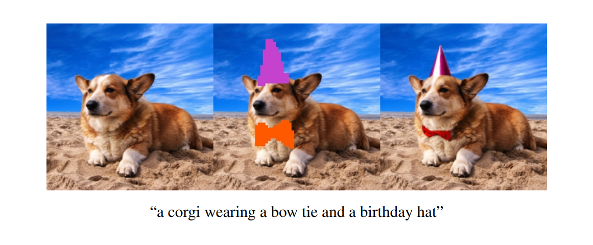
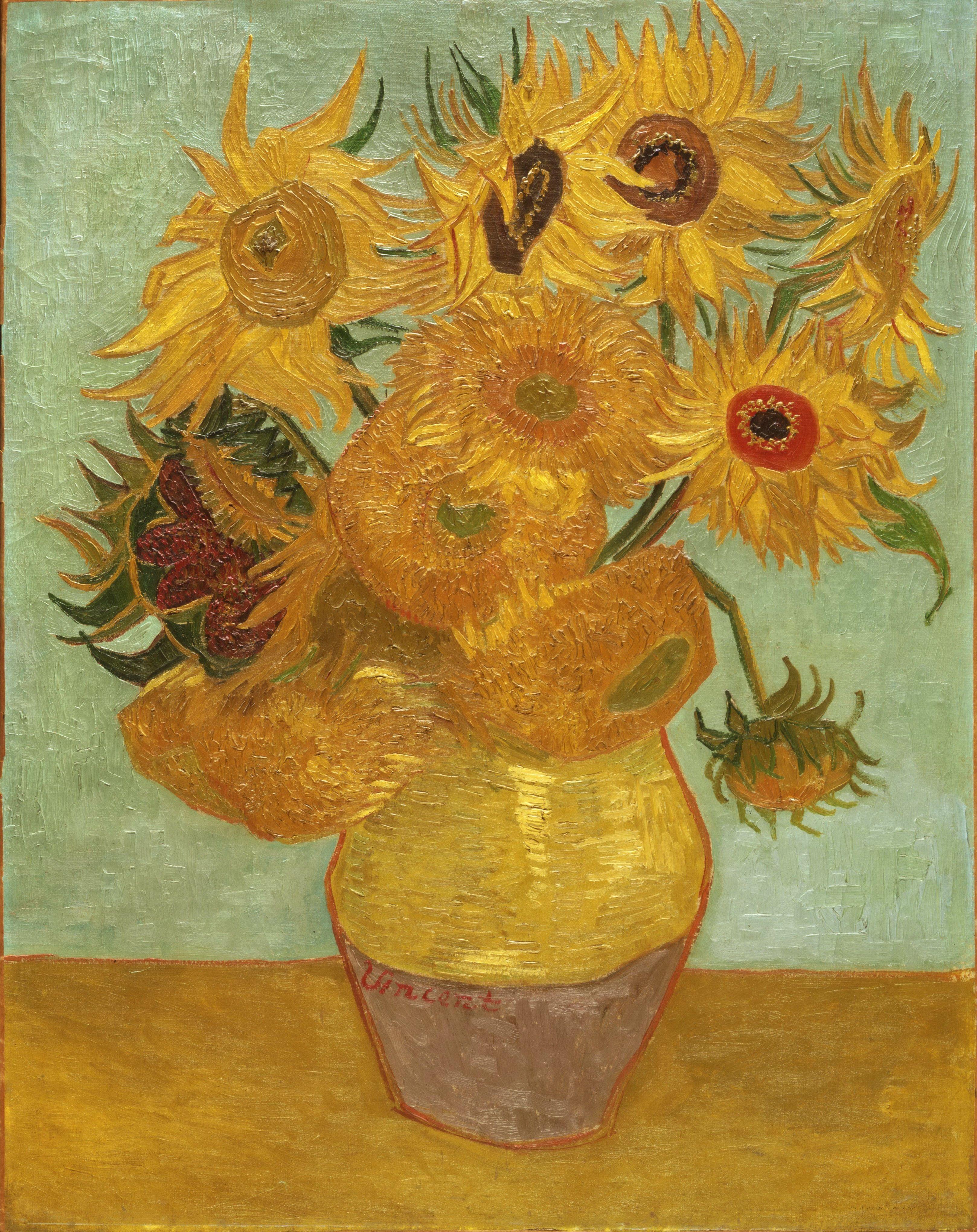
4.4.4 Discussion and prospects
In the last years, methods to generate images via text prompting improved tremendously and a new field of art arised. It is surprising how these models are able to create images only based on a short text instruction. This is quite impressive as AI achieved some level of creativity. It is up for discussion to which extent the computer is becoming the artist in generative arts and in this way replacing the human artist. However, there is still no direct loss function that can calculate how aesthetically pleasing a picture is (Esser, Rombach, and Ommer 2020). This is probably also quite subjective and cannot be answered for everyone in the same way. Most of the time the computer works as aid for the creative process by generating multiple images. Then, the human artist can pick the best outcome or vary the text prompt to improve the output in a desired way. However, the better the AI becomes, the less the human artist needs to intervene in this process.
Furthermore, as the output becomes more and more realistic, there is the risk that these methods are abused to facilitate plagiarism or create fake content and spread misleading information (Dehouche 2021). After all, the outputs look totally realistic, but are completely made-up and generated by the computer. For this reason, some organisations like Open-AI do not release all their models (e.g. DALL-E) or downstream models (e.g. CLIP). On the other hand, from a scientific point of view, it is important to get access to such models to continue research.
Moreover, similarly to most Deep Learning algorithms, these models are affected by biases in the input data (R. Srinivasan and Uchino 2021). For instance, Esser, Rombach, and Ommer (2020) points out that CLIP text embeddings associate a human being more with a man than with a woman. In this way it might be more likely that our models generate a man with the text prompt “human being” than a woman. This effect needs to be further investigated and should be removed.
After all, generative arts can be used to create Non Fungible Tokens (NFT) relatively easily. NFTs are digital artworks where a special digital signature is added making them unique and in this way non-fungible (Wang et al. 2021). The digital artwork is bought and sold online, often by means of cryptocurrency. That is why this field is also called Cryptoart. This provides the perfect platform to sell generative arts. However, this trading market is quite new and controversial, similar to crypotcurrency trading in general.
In conclusion, generative arts is a new and impressive field. It combines technology with arts, two rather opposite fields. The methods are already really impressive and are still getting better and better. For instance, this year Open AI already published DALLE-2 (Ramesh, Dhariwal, et al. 2022a) that outperforms DALLE-1. It remains highly interesting to follow up with the developments in this field.
References
Akbari, Hassan, Liangzhe Yuan, Rui Qian, Wei-Hong Chuang, Shih-Fu Chang, Yin Cui, and Boqing Gong. 2021. “VATT: Transformers for Multimodal Self-Supervised Learning from Raw Video, Audio and Text.” In Advances in Neural Information Processing Systems 34: Annual Conference on Neural Information Processing Systems 2021, Neurips 2021, December 6-14, 2021, Virtual, edited by Marc’Aurelio Ranzato, Alina Beygelzimer, Yann N. Dauphin, Percy Liang, and Jennifer Wortman Vaughan, 24206–21. https://proceedings.neurips.cc/paper/2021/hash/cb3213ada48302953cb0f166464ab356-Abstract.html.
Aran, Komatsuzaki. 2021. “When You Generate Images with Vqgan Clip, the Image Quality Dramatically Improves If You Add "Unreal Engine" to Your Prompt. People Are Now Calling This "Unreal Engine Trick".” Twitter. https://twitter.com/arankomatsuzaki/status/1399471244760649729.
Bachmann, Roman, David Mizrahi, Andrei Atanov, and Amir Zamir. 2022. “MultiMAE: Multi-Modal Multi-Task Masked Autoencoders.” arXiv Preprint arXiv: Arxiv-2204.01678.
Baevski, Alexei, Wei-Ning Hsu, Qiantong Xu, Arun Babu, Jiatao Gu, and Michael Auli. 2022. “Data2vec: A General Framework for Self-Supervised Learning in Speech, Vision and Language.” arXiv Preprint arXiv:2202.03555.
Baltrušaitis, Tadas, Chaitanya Ahuja, and Louis-Philippe Morency. 2017. “Multimodal Machine Learning: A Survey and Taxonomy.” arXiv Preprint arXiv: Arxiv-1705.09406.
Bäck, Thomas, and Hans-Paul Schwefel. 1993. “An Overview of Evolutionary Algorithms for Parameter Optimization.” Evolutionary Computation 1 (1): 1–23. https://doi.org/10.1162/evco.1993.1.1.1.
Bellemare, Marc G., Yavar Naddaf, Joel Veness, and Michael Bowling. 2013. “The Arcade Learning Environment: An Evaluation Platform for General Agents.” J. Artif. Int. Res. 47 (1): 253–79.
Bengio, Yoshua, Aaron C. Courville, and Pascal Vincent. 2013. “Representation Learning: A Review and New Perspectives.” IEEE Trans. Pattern Anal. Mach. Intell. 35 (8): 1798–1828. https://doi.org/10.1109/TPAMI.2013.50.
Boris, Dayma. 2022. “DALL·E Mini.” https://huggingface.co/spaces/dalle-mini/dalle-mini.
Carion, Nicolas, Francisco Massa, Gabriel Synnaeve, Nicolas Usunier, Alexander Kirillov, and Sergey Zagoruyko. 2020. “End-to-End Object Detection with Transformers.” CoRR. https://arxiv.org/abs/2005.12872.
Carreira, Joao, Skanda Koppula, Daniel Zoran, Adria Recasens, Catalin Ionescu, Olivier Henaff, Evan Shelhamer, et al. 2022. “Hierarchical Perceiver.” arXiv Preprint arXiv: Arxiv-2202.10890.
Caruana, Rich. 1997. “Multitask Learning.” Machine Learning 28 (1): 41–75.
Cheerla, Anika, and Olivier Gevaert. 2019. “Deep Learning with Multimodal Representation for Pancancer Prognosis Prediction.” Bioinformatics 35 (14): i446–i454.
Chen, Ting, Simon Kornblith, Mohammad Norouzi, and Geoffrey E. Hinton. 2020b. “A Simple Framework for Contrastive Learning of Visual Representations.” In Proceedings of the 37th International Conference on Machine Learning, ICML 2020, 13-18 July 2020, Virtual Event, 119:1597–1607. Proceedings of Machine Learning Research. PMLR. http://proceedings.mlr.press/v119/chen20j.html.
Cheng, Heng-Tze, Levent Koc, Jeremiah Harmsen, Tal Shaked, Tushar Chandra, Hrishi Aradhye, Glen Anderson, et al. 2016. “Wide & Deep Learning for Recommender Systems.” In Proceedings of the 1st Workshop on Deep Learning for Recommender Systems, 7–10.
Crawshaw, Michael. 2020. “Multi-Task Learning with Deep Neural Networks: A Survey.” arXiv. https://doi.org/10.48550/ARXIV.2009.09796.
Dean, Jeff. 2021. “Introducing Pathways: A Next-Generation Ai Architecture.” 2021. https://blog.google/technology/ai/introducing-pathways-next-generation-ai-architecture/.
Dean, Jeffrey. 2020. “1.1 the Deep Learning Revolution and Its Implications for Computer Architecture and Chip Design.” In 2020 Ieee International Solid- State Circuits Conference - (Isscc), 8–14. https://doi.org/10.1109/ISSCC19947.2020.9063049.
Dehouche, Nassim. 2021. “Plagiarism in the Age of Massive Generative Pre-Trained Transformers (Gpt-3).” Ethics in Science and Environmental Politics 21: 17–23.
Deng, Jia, Wei Dong, Richard Socher, Li-Jia Li, Kai Li, and Li Fei-Fei. 2009. “Imagenet: A Large-Scale Hierarchical Image Database.” In 2009 Ieee Conference on Computer Vision and Pattern Recognition, 248–55. Ieee.
Devlin, Jacob, Ming-Wei Chang, Kenton Lee, and Kristina Toutanova. 2018b. “BERT: Pre-Training of Deep Bidirectional Transformers for Language Understanding.” http://arxiv.org/abs/1810.04805.
Dhariwal, Prafulla, and Alex Nichol. 2021. “Diffusion Models Beat Gans on Image Synthesis.” CoRR. https://arxiv.org/abs/2105.05233.
Doerr, Benjamin, and Frank Neumann. 2021. “A Survey on Recent Progress in the Theory of Evolutionary Algorithms for Discrete Optimization.” ACM Trans. Evol. Learn. Optim. 1 (4). https://doi.org/10.1145/3472304.
Dosovitskiy, Alexey, Lucas Beyer, Alexander Kolesnikov, Dirk Weissenborn, Xiaohua Zhai, Thomas Unterthiner, Mostafa Dehghani, et al. 2020. “An Image Is Worth 16x16 Words: Transformers for Image Recognition at Scale.” arXiv Preprint arXiv:2010.11929.
Dosovitskiy, Alexey, Lucas Beyer, Alexander Kolesnikov, Dirk Weissenborn, Xiaohua Zhai, Thomas Unterthiner, Mostafa Dehghani, et al. 2021. “An Image Is Worth 16x16 Words: Transformers for Image Recognition at Scale.” In 9th International Conference on Learning Representations, ICLR 2021, Virtual Event, Austria, May 3-7, 2021. OpenReview.net. https://openreview.net/forum?id=YicbFdNTTy.
Esser, Patrick, Robin Rombach, and Björn Ommer. 2020. “A Note on Data Biases in Generative Models.” arXiv. https://doi.org/10.48550/ARXIV.2012.02516.
Fernando, Chrisantha, Dylan Banarse, Charles Blundell, Yori Zwols, David Ha, Andrei A. Rusu, Alexander Pritzel, and Daan Wierstra. 2017. “PathNet: Evolution Channels Gradient Descent in Super Neural Networks.” In. https://arxiv.org/abs/1701.08734.
Galanter, Philip. 2016. “Generative Art Theory.” A Companion to Digital Art 1: 631.
Gatys, Leon A., Alexander S. Ecker, and Matthias Bethge. 2016. “A Neural Algorithm of Artistic Style.” arXiv. https://doi.org/10.48550/ARXIV.1508.06576.
Gebru, Timnit, Jonathan Krause, Yilun Wang, Duyun Chen, Jia Deng, Erez Aiden, and Li Fei-Fei. 2017. “Using Deep Learning and Google Street View to Estimate the Demographic Makeup of Neighborhoods Across the United States.” Proceedings of the National Academy of Sciences 114: 201700035. https://doi.org/10.1073/pnas.1700035114.
Gesmundo, Andrea, and Jeff Dean. 2022. “MuNet: Evolving Pretrained Deep Neural Networks into Scalable Auto-Tuning Multitask Systems.” arXiv. https://doi.org/10.48550/ARXIV.2205.10937.
Goodfellow, Ian, Jean Pouget-Abadie, Mehdi Mirza, Bing Xu, David Warde-Farley, Sherjil Ozair, Aaron Courville, and Yoshua Bengio. 2014. “Generative Adversarial Nets.” In Advances in Neural Information Processing Systems, edited by Z. Ghahramani, M. Welling, C. Cortes, N. Lawrence, and K. Q. Weinberger. Vol. 27. Curran Associates, Inc. https://proceedings.neurips.cc/paper/2014/file/5ca3e9b122f61f8f06494c97b1afccf3-Paper.pdf.
Grill, Jean-Bastien, Florian Strub, Florent Altch’e, Corentin Tallec, Pierre H. Richemond, Elena Buchatskaya, Carl Doersch, et al. 2020. “Bootstrap Your Own Latent: A New Approach to Self-Supervised Learning.” Neurips.
He, Kaiming, Xiangyu Zhang, Shaoqing Ren, and Jian Sun. 2015. “Deep Residual Learning for Image Recognition.” CoRR. http://arxiv.org/abs/1512.03385.
Hinton, Geoffrey, Oriol Vinyals, and Jeff Dean. 2015. “Distilling the Knowledge in a Neural Network.” arXiv. https://doi.org/10.48550/ARXIV.1503.02531.
Ho, Jonathan, Ajay Jain, and Pieter Abbeel. 2020b. “Denoising Diffusion Probabilistic Models.” In Advances in Neural Information Processing Systems 33: Annual Conference on Neural Information Processing Systems 2020, Neurips 2020, December 6-12, 2020, Virtual, edited by Hugo Larochelle, Marc’Aurelio Ranzato, Raia Hadsell, Maria-Florina Balcan, and Hsuan-Tien Lin. https://proceedings.neurips.cc/paper/2020/hash/4c5bcfec8584af0d967f1ab10179ca4b-Abstract.html.
Hu, Ronghang, and Amanpreet Singh. 2021b. “UniT: Multimodal Multitask Learning with a Unified Transformer.” In 2021 Ieee/Cvf International Conference on Computer Vision (Iccv), 1419–29. https://doi.org/10.1109/ICCV48922.2021.00147.
Huang, Shih-Cheng, Anuj Pareek, Saeed Seyyedi, Imon Banerjee, and Matthew P Lungren. 2020. “Fusion of Medical Imaging and Electronic Health Records Using Deep Learning: A Systematic Review and Implementation Guidelines.” NPJ Digital Medicine 3 (1): 1–9.
IV, William C. Sleeman, Rishabh Kapoor, and Preetam Ghosh. 2021. “Multimodal Classification: Current Landscape, Taxonomy and Future Directions.” arXiv Preprint arXiv: Arxiv-2109.09020.
Jacobs, Robert A., Michael I. Jordan, Steven J. Nowlan, and Geoffrey E. Hinton. 1991. “Adaptive Mixtures of Local Experts.” Neural Computation 3 (1): 79–87. https://doi.org/10.1162/neco.1991.3.1.79.
Jaegle, Andrew, Felix Gimeno, Andy Brock, Oriol Vinyals, Andrew Zisserman, and Joao Carreira. 2021a. “Perceiver: General Perception with Iterative Attention.” In International Conference on Machine Learning, 4651–64. PMLR.
Jaegle, Andrew, Felix Gimeno, Andy Brock, Oriol Vinyals, Andrew Zisserman, and João Carreira. 2021b. “Perceiver: General Perception with Iterative Attention.” In Proceedings of the 38th International Conference on Machine Learning, ICML 2021, 18-24 July 2021, Virtual Event, edited by Marina Meila and Tong Zhang, 139:4651–64. Proceedings of Machine Learning Research. PMLR. http://proceedings.mlr.press/v139/jaegle21a.html.
Jean, Neal, Marshall Burke, Michael Xie, W. Matthew Davis, David B. Lobell, and Stefano Ermon. 2016. “Combining Satellite Imagery and Machine Learning to Predict Poverty.” Science 353 (6301): 790–94. https://doi.org/10.1126/science.aaf7894.
Jordan, Michael I., and Robert A. Jacobs. 1994. “Hierarchical Mixtures of Experts and the Em Algorithm.” Neural Computation 6 (2): 181–214. https://doi.org/10.1162/neco.1994.6.2.181.
Kahatapitiya, Kumara, and Michael S. Ryoo. 2021. “SWAT: Spatial Structure Within and Among Tokens.” arXiv Preprint arXiv: Arxiv-2111.13677.
Kaiser, Lukasz, Aidan N. Gomez, Noam Shazeer, Ashish Vaswani, Niki Parmar, Llion Jones, and Jakob Uszkoreit. 2017. “One Model to Learn Them All.” arXiv. https://arxiv.org/pdf/1706.05137.pdf.
Karras, Tero, Samuli Laine, and Timo Aila. 2019. “A Style-Based Generator Architecture for Generative Adversarial Networks.” In Proceedings of the Ieee/Cvf Conference on Computer Vision and Pattern Recognition, 4401–10.
Katzman, Jared L, Uri Shaham, Alexander Cloninger, Jonathan Bates, Tingting Jiang, and Yuval Kluger. 2018. “DeepSurv: Personalized Treatment Recommender System Using a Cox Proportional Hazards Deep Neural Network.” BMC Medical Research Methodology 18 (1): 1–12.
Kopper, Philipp, Simon Wiegrebe, Bernd Bischl, Andreas Bender, and David Rügamer. 2022. “DeepPAMM: Deep Piecewise Exponential Additive Mixed Models for Complex Hazard Structures in Survival Analysis.” In Pacific-Asia Conference on Knowledge Discovery and Data Mining, 249–61. Springer.
Kudo, Taku, and John Richardson. 2018. “SentencePiece: A Simple and Language Independent Subword Tokenizer and Detokenizer for Neural Text Processing.” In Proceedings of the 2018 Conference on Empirical Methods in Natural Language Processing: System Demonstrations, 66–71. Brussels, Belgium: Association for Computational Linguistics. https://doi.org/10.18653/v1/D18-2012.
Law, Stephen, Brooks Paige, and Chris Russell. 2019. “Take a Look Around.” ACM Transactions on Intelligent Systems and Technology 10 (5): 1–19. https://doi.org/10.1145/3342240.
LeCun, Yann. 2022. “A Path Towards Autonomous Machine Intelligence Version 0.9. 2, 2022-06-27.”
Lewis, Mike, Yinhan Liu, Naman Goyal, Marjan Ghazvininejad, Abdelrahman Mohamed, Omer Levy, Veselin Stoyanov, and Luke Zettlemoyer. 2020. “BART: Denoising Sequence-to-Sequence Pre-Training for Natural Language Generation, Translation, and Comprehension.” In Proceedings of the 58th Annual Meeting of the Association for Computational Linguistics, 7871–80. Online: Association for Computational Linguistics. https://doi.org/10.18653/v1/2020.acl-main.703.
Lewkowycz, Aitor, Anders Andreassen, David Martin Dohan, Ethan S Dyer, Henryk Michalewski, Vinay Ramasesh, Ambrose Slone, et al. 2022. “Solving Quantitative Reasoning Problems with Language Models.” Technical report. https://arxiv.org/abs/2206.14858.
Lin, Tsung-Yi, Michael Maire, Serge Belongie, James Hays, Pietro Perona, Deva Ramanan, Piotr Dollár, and C. Lawrence Zitnick. 2014b. “Microsoft Coco: Common Objects in Context.” In Computer Vision – Eccv 2014, 740–55. Springer International Publishing.
Mccormack, Jon, and Camilo Cruz Gambardella. 2022. “Growing and Evolving 3-d Prints.” IEEE Transactions on Evolutionary Computation 26 (1): 88–99. https://doi.org/10.1109/TEVC.2021.3095156.
Mordvintsev, Alexander. 2015. “Inceptionism: Going Deeper into Neural Networks.” Google AI Blog. Google. https://ai.googleblog.com/2015/06/inceptionism-going-deeper-into-neural.html.
Mustafa, Basil, Carlos Riquelme, Joan Puigcerver, Rodolphe Jenatton, and Neil Houlsby. 2022. “Multimodal Contrastive Learning with Limoe: The Language-Image Mixture of Experts.” arXiv. https://doi.org/10.48550/ARXIV.2206.02770.
Nagrani, Arsha, Shan Yang, Anurag Arnab, Aren Jansen, Cordelia Schmid, and Chen Sun. 2021. “Attention Bottlenecks for Multimodal Fusion.” In Advances in Neural Information Processing Systems 34: Annual Conference on Neural Information Processing Systems 2021, Neurips 2021, December 6-14, 2021, Virtual, edited by Marc’Aurelio Ranzato, Alina Beygelzimer, Yann N. Dauphin, Percy Liang, and Jennifer Wortman Vaughan, 14200–14213. https://proceedings.neurips.cc/paper/2021/hash/76ba9f564ebbc35b1014ac498fafadd0-Abstract.html.
Nichol, Alex, Prafulla Dhariwal, Aditya Ramesh, Pranav Shyam, Pamela Mishkin, Bob McGrew, Ilya Sutskever, and Mark Chen. 2021a. “GLIDE: Towards Photorealistic Image Generation and Editing with Text-Guided Diffusion Models.” arXiv. https://doi.org/10.48550/ARXIV.2112.10741.
OpenAI. 2021. “DALL-E.” https://github.com/openai/DALL-E.
Patashnik, Or, Zongze Wu, Eli Shechtman, Daniel Cohen-Or, and Dani Lischinski. 2021. “StyleCLIP: Text-Driven Manipulation of Stylegan Imagery.” CoRR. https://arxiv.org/abs/2103.17249.
Pölsterl, Sebastian, Ignacio Sarasua, Benjamı́n Gutiérrez-Becker, and Christian Wachinger. 2019. “A Wide and Deep Neural Network for Survival Analysis from Anatomical Shape and Tabular Clinical Data.” In Joint European Conference on Machine Learning and Knowledge Discovery in Databases, 453–64. Springer.
Qiao, Han, Vivian Liu, and Lydia Chilton. 2022. “Initial Images: Using Image Prompts to Improve Subject Representation in Multimodal Ai Generated Art.” In Creativity and Cognition, 15–28.
Radford, Alec, Jong Wook Kim, Chris Hallacy, Aditya Ramesh, Gabriel Goh, Sandhini Agarwal, Girish Sastry, et al. 2021a. “Learning Transferable Visual Models from Natural Language Supervision.” arXiv. https://doi.org/10.48550/ARXIV.2103.00020.
Radford, Alec, Jong Wook Kim, Chris Hallacy, Aditya Ramesh, Gabriel Goh, Sandhini Agarwal, Girish Sastry, et al. 2021b. “Learning Transferable Visual Models from Natural Language Supervision.” In Proceedings of the 38th International Conference on Machine Learning, ICML 2021, 18-24 July 2021, Virtual Event, edited by Marina Meila and Tong Zhang, 139:8748–63. Proceedings of Machine Learning Research. PMLR. http://proceedings.mlr.press/v139/radford21a.html.
Radford, Alec, Jong Wook Kim, Chris Hallacy, Aditya Ramesh, Gabriel Goh, Sandhini Agarwal, Girish Sastry, et al. 2021. “Learning Transferable Visual Models from Natural Language Supervision.” In International Conference on Machine Learning, 8748–63. PMLR.
Ramesh, Aditya, Prafulla Dhariwal, Alex Nichol, Casey Chu, and Mark Chen. 2022a. “Hierarchical Text-Conditional Image Generation with Clip Latents.” arXiv. https://doi.org/10.48550/ARXIV.2204.06125.
Ramesh, Aditya, Mikhail Pavlov, Gabriel Goh, Scott Gray, Chelsea Voss, Alec Radford, Mark Chen, and Ilya Sutskever. 2021a. “Zero-Shot Text-to-Image Generation.” arXiv. https://doi.org/10.48550/ARXIV.2102.12092.
Ramesh, Aditya, Mikhail Pavlov, Gabriel Goh, Scott Gray, Chelsea Voss, Alec Radford, Mark Chen, and Ilya Sutskever. 2021c. “Zero-Shot Text-to-Image Generation.” In Proceedings of the 38th International Conference on Machine Learning, ICML 2021, 18-24 July 2021, Virtual Event, edited by Marina Meila and Tong Zhang, 139:8821–31. Proceedings of Machine Learning Research. PMLR. http://proceedings.mlr.press/v139/ramesh21a.html.
Ramesh, Aditya, Mikhail Pavlov, Gabriel Goh, Scott Gray, Chelsea Voss, Alec Radford, Mark Chen, and Ilya Sutskever. 2021d. “Zero-Shot Text-to-Image Generation.” In Proceedings of the 38th International Conference on Machine Learning, edited by Marina Meila and Tong Zhang, 139:8821–31. Proceedings of Machine Learning Research. PMLR. https://proceedings.mlr.press/v139/ramesh21a.html.
Rebuffi, Sylvestre-Alvise, Hakan Bilen, and Andrea Vedaldi. 2017. “Learning Multiple Visual Domains with Residual Adapters.” In Advances in Neural Information Processing Systems, edited by I. Guyon, U. Von Luxburg, S. Bengio, H. Wallach, R. Fergus, S. Vishwanathan, and R. Garnett. Vol. 30. Curran Associates, Inc. https://proceedings.neurips.cc/paper/2017/file/e7b24b112a44fdd9ee93bdf998c6ca0e-Paper.pdf.
Reed, Scott, Konrad Zolna, Emilio Parisotto, Sergio Gomez Colmenarejo, Alexander Novikov, Gabriel Barth-Maron, Mai Gimenez, et al. 2022. “A Generalist Agent.” arXiv. https://doi.org/10.48550/ARXIV.2205.06175.
Riquelme, Carlos, Joan Puigcerver, Basil Mustafa, Maxim Neumann, Rodolphe Jenatton, André Susano Pinto, Daniel Keysers, and Neil Houlsby. 2021. “Scaling Vision with Sparse Mixture of Experts.” In Advances in Neural Information Processing Systems, edited by M. Ranzato, A. Beygelzimer, Y. Dauphin, P. S. Liang, and J. Wortman Vaughan, 34:8583–95. Curran Associates, Inc. https://proceedings.neurips.cc/paper/2021/file/48237d9f2dea8c74c2a72126cf63d933-Paper.pdf.
Russakovsky, Olga, Jia Deng, Hao Su, Jonathan Krause, Sanjeev Satheesh, Sean Ma, Zhiheng Huang, et al. 2015. “ImageNet Large Scale Visual Recognition Challenge.” Int. J. Comput. Vision 115 (3): 211–52. https://doi.org/10.1007/s11263-015-0816-y.
Rügamer, David, Chris Kolb, and Nadja Klein. 2020. “Semi-Structured Deep Distributional Regression: Combining Structured Additive Models and Deep Learning.” arXiv Preprint arXiv:2002.05777.
Saharia, Chitwan, William Chan, Saurabh Saxena, Lala Li, Jay Whang, Emily Denton, Seyed Kamyar Seyed Ghasemipour, et al. 2022a. “Photorealistic Text-to-Image Diffusion Models with Deep Language Understanding.” arXiv Preprint arXiv: Arxiv-2205.11487.
Schuhmann, Christoph, Richard Vencu, Romain Beaumont, Robert Kaczmarczyk, Clayton Mullis, Aarush Katta, Theo Coombes, Jenia Jitsev, and Aran Komatsuzaki. 2021b. “LAION-400M: Open Dataset of Clip-Filtered 400 Million Image-Text Pairs.” CoRR. https://arxiv.org/abs/2111.02114.
Sennrich, Rico, Barry Haddow, and Alexandra Birch. 2016. “Neural Machine Translation of Rare Words with Subword Units.” In Proceedings of the 54th Annual Meeting of the Association for Computational Linguistics (Volume 1: Long Papers), 1715–25. Berlin, Germany: Association for Computational Linguistics. https://doi.org/10.18653/v1/P16-1162.
Shazeer, Noam, Azalia Mirhoseini, Krzysztof Maziarz, Andy Davis, Quoc Le, Geoffrey Hinton, and Jeff Dean. 2017. “Outrageously Large Neural Networks: The Sparsely-Gated Mixture-of-Experts Layer.” In. https://openreview.net/pdf?id=B1ckMDqlg.
Shonenkov, Alex. 2021. “RuDALL-E.” https://github.com/ai-forever/ru-dalle.
Shvetsova, Nina, Brian Chen, Andrew Rouditchenko, Samuel Thomas, Brian Kingsbury, Rogerio Feris, David Harwath, James Glass, and Hilde Kuehne. 2021. “Everything at Once - Multi-Modal Fusion Transformer for Video Retrieval.” arXiv Preprint arXiv: Arxiv-2112.04446.
Sirko, Wojciech, Sergii Kashubin, Marvin Ritter, Abigail Annkah, Yasser Salah Eddine Bouchareb, Yann N. Dauphin, Daniel Keysers, Maxim Neumann, Moustapha Cissé, and John Quinn. 2021. “Continental-Scale Building Detection from High Resolution Satellite Imagery.” CoRR. https://arxiv.org/abs/2107.12283.
Soderlund, Jacob, and Alan Blair. 2018. “Adversarial Image Generation Using Evolution and Deep Learning.” In 2018 Ieee Congress on Evolutionary Computation (Cec), 1–8. https://doi.org/10.1109/CEC.2018.8477754.
Srinivasan, Ramya, and Kanji Uchino. 2021. “Biases in Generative Art: A Causal Look from the Lens of Art History.” In Proceedings of the 2021 Acm Conference on Fairness, Accountability, and Transparency, 41–51.
Steiner, Andreas, Alexander Kolesnikov, Xiaohua Zhai, Ross Wightman, Jakob Uszkoreit, and Lucas Beyer. 2021. “How to Train Your Vit? Data, Augmentation, and Regularization in Vision Transformers.” https://doi.org/10.48550/ARXIV.2106.10270.
Sulubacak, Umut, Ozan Caglayan, Stig-Arne Grönroos, Aku Rouhe, Desmond Elliott, Lucia Specia, and Jörg Tiedemann. 2020. “Multimodal Machine Translation Through Visuals and Speech.” Mach. Transl. 34 (2-3): 97–147. https://doi.org/10.1007/s10590-020-09250-0.
Tong, Chao, Jun Li, Chao Lang, Fanxin Kong, Jianwei Niu, and Joel JPC Rodrigues. 2018. “An Efficient Deep Model for Day-Ahead Electricity Load Forecasting with Stacked Denoising Auto-Encoders.” Journal of Parallel and Distributed Computing 117: 267–73.
Vale-Silva, Luı́s A, and Karl Rohr. 2021. “Long-Term Cancer Survival Prediction Using Multimodal Deep Learning.” Scientific Reports 11 (1): 1–12.
Vaswani, Ashish, Noam Shazeer, Niki Parmar, Jakob Uszkoreit, Llion Jones, Aidan N. 2017c. “Attention Is All You Need.” In Advances in Neural Information Processing Systems 30: Annual Conference on Neural Information Processing Systems 2017, December 4-9, 2017, Long Beach, ca, USA, edited by Isabelle Guyon, Ulrike von Luxburg, Samy Bengio, Hanna M. Wallach, Rob Fergus, S. V. N. Vishwanathan, and Roman Garnett, 5998–6008. https://proceedings.neurips.cc/paper/2017/hash/3f5ee243547dee91fbd053c1c4a845aa-Abstract.html.
Vaswani, Ashish, Noam Shazeer, Niki Parmar, Jakob Uszkoreit, Llion Jones, Aidan N Gomez, Łukasz Kaiser, and Illia Polosukhin. 2017b. “Attention Is All You Need.” Advances in Neural Information Processing Systems 30.
Wang, Peng, An Yang, Rui Men, Junyang Lin, Shuai Bai, Zhikang Li, Jianxin Ma, Chang Zhou, Jingren Zhou, and Hongxia Yang. 2022. “OFA: Unifying Architectures, Tasks, and Modalities Through a Simple Sequence-to-Sequence Learning Framework.” In Proceedings of the 39th International Conference on Machine Learning, edited by Kamalika Chaudhuri, Stefanie Jegelka, Le Song, Csaba Szepesvari, Gang Niu, and Sivan Sabato, 162:23318–40. Proceedings of Machine Learning Research. PMLR. https://proceedings.mlr.press/v162/wang22al.html.
Wang, Qin, Rujia Li, Qi Wang, and Shiping Chen. 2021. “Non-Fungible Token (Nft): Overview, Evaluation, Opportunities and Challenges.” arXiv. https://doi.org/10.48550/ARXIV.2105.07447.
Wu, Chenfei, Jian Liang, Lei Ji, Fan Yang, Yuejian Fang, Daxin Jiang, and Nan Duan. 2021. “NÜWA: Visual Synthesis Pre-Training for Neural visUal World creAtion.” arXiv Preprint arXiv: Arxiv-2111.12417.
WZRD. 2020. “WZRD.” https://wzrd.ai/.
Yao, Jiawen, Xinliang Zhu, Feiyun Zhu, and Junzhou Huang. 2017. “Deep Correlational Learning for Survival Prediction from Multi-Modality Data.” In Medical Image Computing and Computer-Assisted Intervention − Miccai 2017, 406–14. Springer International Publishing.
You, Jiaxuan, Xiaocheng Li, Melvin Low, David Lobell, and Stefano Ermon. 2017. “Deep Gaussian Process for Crop Yield Prediction Based on Remote Sensing Data.” In Proceedings of the Thirty-First Aaai Conference on Artificial Intelligence, 4559–65. AAAI’17. San Francisco, California, USA: AAAI Press.
Yu, Jiahui, Yuanzhong Xu, Jing Koh, Thang Luong, Gunjan Baid, Vijay Vasudevan, Alexander Ku, et al. 2022a. “Scaling Autoregressive Models for Content-Rich Text-to-Image Generation.” https://doi.org/10.48550/arXiv.2206.10789.
Zhang, Chao, Zichao Yang, Xiaodong He, and Li Deng. 2020. “Multimodal Intelligence: Representation Learning, Information Fusion, and Applications.” IEEE J. Sel. Top. Signal Process. 14 (3): 478–93. https://doi.org/10.1109/JSTSP.2020.2987728.
Zhu, Xinliang, Jiawen Yao, and Junzhou Huang. 2016. “Deep Convolutional Neural Network for Survival Analysis with Pathological Images.” In 2016 Ieee International Conference on Bioinformatics and Biomedicine (Bibm), 544–47. IEEE.