Chapter 2 Introducing the modalities

Authors: Cem Akkus, Vladana Djakovic, Christopher Benjamin Marquardt

Supervisor: Matthias Aßenmacher

Natural Language Processing (NLP) has existed for about 50 years, but it is more relevant than ever. There have been several breakthroughs in this branch of machine learning that is concerned with spoken and written language. For example, learning internal representations of words was one of the greater advances of the last decade. Word embeddings (Mikolov, Chen, et al. (2013 a), Bojanowski et al. (2016)) made it possible and allowed developers to encode words as dense vectors that capture their underlying semantic content. In this way, similar words are embedded close to each other in a lower-dimensional feature space. Another important challenge was solved by Encoder-decoder (also called sequence-to-sequence) architectures Sutskever, Vinyals, and Le (2014), which made it possible to map input sequences to output sequences of different lengths. They are especially useful for complex tasks like machine translation, video captioning or question answering. This approach makes minimal assumptions on the sequence structure and can deal with different word orders and active, as well as passive voice.

A definitely significant state-of-the-art technique is Attention Bahdanau, Cho, and Bengio (2014), which enables models to actively shift their focus – just like humans do. It allows following one thought at a time while suppressing information irrelevant to the task. As a consequence, it has been shown to significantly improve performance for tasks like machine translation. By giving the decoder access to directly look at the source, the bottleneck is avoided and at the same time, it provides a shortcut to faraway states and thus helps with the vanishing gradient problem. One of the most recent sequence data modeling techniques is Transformers (Vaswani, Shazeer, Parmar, Uszkoreit, Jones, Gomez, Kaiser, et al. (2017 b)), which are solely based on attention and do not have to process the input data sequentially (like RNNs). Therefore, the deep learning model is better in remembering context-induced earlier in long sequences. It is the dominant paradigm in NLP currently and even makes better use of GPUs, because it can perform parallel operations. Transformer architectures like BERT (Devlin et al. 2018 b), T5 (Raffel et al. 2019 a) or GPT-3 (Brown et al. 2020) are pre-trained on a large corpus and can be fine-tuned for specific language tasks. They have the capability to generate stories, poems, code and much more. With the help of the aforementioned breakthroughs, deep networks have been successful in retrieving information and finding representations of semantics in the modality text. In the next paragraphs, developments for another modality image are going to be presented.

Computer vision (CV) focuses on replicating parts of the complexity of the human visual system and enabling computers to identify and process objects in images and videos in the same way that humans do. In recent years it has become one of the main and widely applied fields of computer science. However, there are still problems that are current research topics, whose solutions depend on the research’s view on the topic. One of the problems is how to optimize deep convolutional neural networks for image classification. The accuracy of classification depends on width, depth and image resolution. One way to address the degradation of training accuracy is by introducing a deep residual learning framework (He et al. 2015). On the other hand, another less common method is to scale up ConvNets, to achieve better accuracy is by scaling up image resolution. Based on this observation, there was proposed a simple yet effective compound scaling method, called EfficientNets (M. Tan and Le 2019 a).

Another state-of-the-art trend in computer vision is learning effective visual representations without human supervision. Discriminative approaches based on contrastive learning in the latent space have recently shown great promise, achieving state-of-the-art results, but the simple framework for contrastive learning of visual representations, which is called SimCLR, outperforms previous work (T. Chen, Kornblith, Norouzi, and Hinton 2020 a). However, another research proposes as an alternative a simple “swapped” prediction problem where we predict the code of a view from the representation of another view. Where features are learned by Swapping Assignments between multiple Views of the same image (SwAV) (Caron et al. 2020). Further recent contrastive methods are trained by reducing the distance between representations of different augmented views of the same image (‘positive pairs’) and increasing the distance between representations of augmented views from different images (‘negative pairs’). Bootstrap Your Own Latent (BYOL) is a new algorithm for self-supervised learning of image representatios (Grill, Strub, Altché, et al. 2020).

Self-attention-based architectures, in particular, Transformers have become the model of choice in natural language processing (NLP). Inspired by NLP successes, multiple works try combining CNN-like architectures with self-attention, some replacing the convolutions entirely. The latter models, while theoretically efficient, have not yet been scaled effectively on modern hardware accelerators due to the use of specialized attention patterns. Inspired by the Transformer scaling successes in NLP, one of the experiments is applying a standard Transformer directly to the image (Dosovitskiy, Beyer, Kolesnikov, Weissenborn, Zhai, Unterthiner, Dehghani, Minderer, Heigold, Gelly, Uszkoreit, et al. 2020 a). Due to the widespread application of computer vision, these problems differ and are constantly being at the center of attention of more and more research.

With the rapid development in NLP and CV in recent years, it was just a question of time to merge both modalities to tackle multi-modal tasks. The release of DALL-E 2 just hints at what one can expect from this merge in the future. DALL-E 2 is able to create photorealistic images or even art from any given text input. So it takes the information of one modality and turns it into another modality. It needs multi-modal datasets to make this possible, which are still relatively rare. This shows the importance of available data and the ability to use it even more. Nevertheless, all modalities are in need of huge datasets to pre-train their models. It’s common to pre-train a model and fine-tune it afterwards for a specific task on another dataset. For example, every state-of-the-art CV model uses a classifier pre-trained on an ImageNet based dataset. The cardinality of the datasets used for CV is immense, but the datasets used for NLP are of a completely different magnitude. BERT uses the English Wikipedia and the Bookscorpus to pre-train the model. The latter consists of almost 1 billion words and 74 million sentences. The pre-training of GPT-3 is composed of five huge corpora: CommonCrawl, Books1 and Books2, Wikipedia and WebText2. Unlike language model pre-training that can leverage tremendous natural language data, vision-language tasks require high-quality image descriptions that are hard to obtain for free. Widely used pre-training datasets for VL-PTM are Microsoft Common Objects in Context (COCO), Visual Genome (VG), Conceptual Captions (CC), Flickr30k, LAION-400M and LAION-5B, which is now the biggest openly accessible image-text dataset.

Besides the importance of pre-training data, there must also be a way to test or compare the different models. A reasonable approach is to compare the performance on specific tasks, which is called benchmarking. A nice feature of benchmarks is that they allow us to compare the models to a human baseline. Different metrics are used to compare the performance of the models. Accuracy is widely used, but there are also some others. For CV the most common benchmark datasets are ImageNet, ImageNetReaL, CIFAR-10(0), OXFORD-IIIT PET, OXFORD Flower 102, COCO and Visual Task Adaptation Benchmark (VTAB). The most common benchmarks for NLP are General Language Understanding Evaluation (GLUE), SuperGLUE, SQuAD 1.1, SQuAD 2.0, SWAG, RACE, ReCoRD, and CoNLL-2003. VTAB, GLUE and SuperGLUE also provide a public leader board. Cross-modal tasks such as Visual Question Answering (VQA), Visual Commonsense Reasoning (VCR), Natural Language Visual Reasoning (NLVR), Flickr30K, COCO and Visual Entailment are common benchmarks for VL-PTM.

2.1 State-of-the-art in NLP

Author: Cem Akkus

Supervisor: Matthias Aßenmacher

2.1.1 Introduction

Natural Language Processing (NLP) exists for about 50 years, but it is more relevant than ever. There have been several breakthroughs in this branch of machine learning that is concerned with spoken and written language. In this work, the most influential ones of the last decade are going to be presented. Starting with word embeddings, which efficiently model word semantics. Encoder-decoder architectures represent another step forward by making minimal assumptions about the sequence structure. Next, the attention mechanism allows human-like focus shifting to put more emphasis on more relevant parts. Then, the transformer applies attention in its architecture to process the data non-sequentially, which boosts the performance on language tasks to exceptional levels. At last, the most influential transformer architectures are recognized before a few current topics in natural language processing are discussed.

2.1.2 Word Embeddings

As mentioned in the introduction, one of the earlier advances in NLP is learning word internal representations. Before that, a big problem with text modelling was its messiness, while machine learning algorithms undoubtedly prefer structured and well-defined fixed-length inputs. On a granular level, the models rather work with numerical than textual data. Thus, by using very basic techniques like one-hot encoding or bag-of-words, a text is converted into its equivalent vector of numbers without losing information.

In the example depicting one-hot encoding (see Figure 2.1), there are ten simple words and the dark squares indicate the only index with a non-zero value.

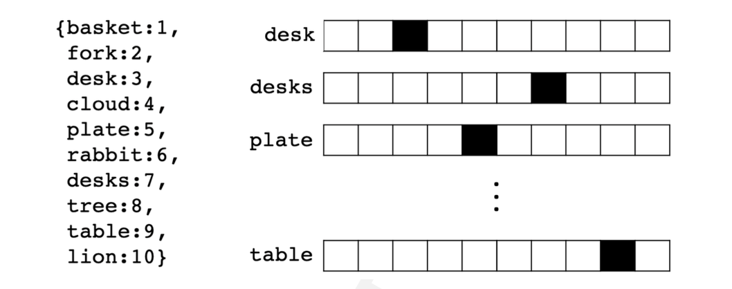
FIGURE 2.1: Ten one-hot encoded words (Source: Pilehvar and Camacho-Collados (2021))

In contrast, there are multiple non-zero values while using bag-of-words, which is another way of extracting features from text to use in modelling where we measure if a word is present from a vocabulary of known words. It is called bag-of-words because the order is disregarded here.

Treating words as atomic units has some plausible reasons, like robustness and simplicity. It was even argued that simple models on a huge amount of data outperform complex models trained on less data. However, simple techniques are problematic for many tasks, e.g. when it comes to relevant in-domain data for automatic speech recognition. The size of high-quality transcribed speech data is often limited to just millions of words, so simply scaling up simpler models is not possible in certain situations and therefore more advanced techniques are needed. Additionally, thanks to the progress of machine learning techniques, it is realistic to train more complex models on massive amounts of data. Logically, more complex models generally outperform basic ones. Other disadvantages of classic word representations are described by the curse of dimensionality and the generalization problem. The former becomes a problem due to the growing vocabulary equivalently increasing the feature size. This results in sparse and high-dimensional vectors. The latter occurs because the similarity between words is not captured. Therefore, previously learned information cannot be used. Besides, assigning a distinct vector to each word is a limitation, which becomes especially obvious for languages with large vocabularies and many rare words.

To combat the downfalls of simple word representations, word embeddings enable to use efficient and dense representations in which similar words have a similar encoding. So words that are closer in the vector space are expected to be similar in meaning. An embedding is hereby defined as a vector of floating point values (with the length of the vector being a hyperparameter). The values for the embedding are trainable parameters which are learned similarly to a model learning the weights for a dense layer. The dimensionality of the word representations is typically much smaller than the number of words in the dictionary. For example, Mikolov, Chen, et al. (2013 a) called dimensions between 50-100 modest for more than a few hundred million words. For small data sets, dimensionality for the word vectors could start at 8 and go up to 1024 for larger data sets. It is expected that higher dimensions can rather pick up intricate relationships between words if given enough data to learn from.

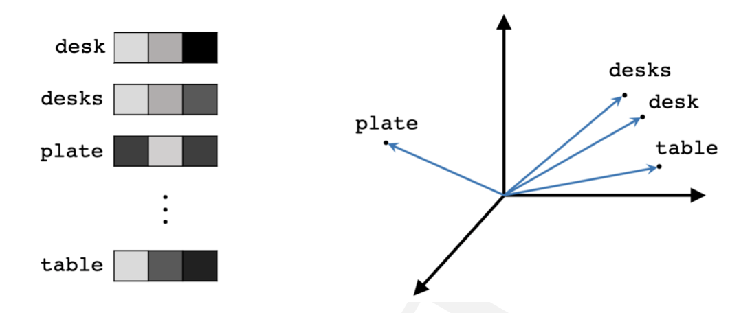
FIGURE 2.2: Three-dimensional word embeddings (Source: Pilehvar and Camacho-Collados (2021)).

For any NLP tasks, it is sensible to start with word embeddings because it allows to conveniently incorporate prior knowledge into the model and can be seen as a basic form of transfer learning. It is important to note that even though embeddings attempt to represent the meaning of words and do that to an extent, the semantics of the word in a given context cannot be captured. This is due to the words having static precomputed representations in traditional embedding techniques. Thus, the word "bank" can either refer to a financial institution or a river bank. Contextual embedding methods offer a solution, but more about them will follow later.

It should be noted that words can have various degrees of similarity. In the context of inflectional languages, it becomes obvious because words are adjusted to articulate grammatical categories. For example, in a subspace of the original vector, nouns that have similar endings can be found. However, it even exceeds simple syntactic regularities. With straightforward operations on the word vectors, it can be displayed that $vector(\text{King}) - vector(\text{Man}) + vector(\text{Woman})$ equals a vector that is closest in vector space (and therefore in meaning) to the word "Queen". A simple visualization of this relationship can be seen in the left graph below (see Figure 2.3). The three coordinate systems are representations of higher dimensions that are depicted in this way via dimension reduction techniques. Furthermore, the verb-to-tense relationship is expressed in the middle graphic, which extends the insight from before referring to the word endings being similar because in this instance the past tenses of both verbs walking and swimming are not similar in structure. Additionally, on the right side of the figure, there is a form of the commonly portrayed and easily understood Country-Capital example (see Mikolov, Chen, et al. (2013 a)).

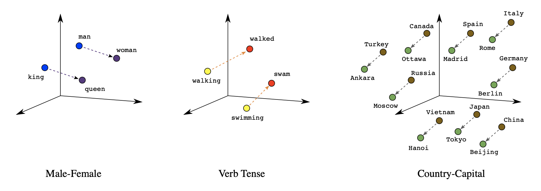
FIGURE 2.3: Three types of similarities as word embeddings (Source: Google (2022)).

Another way of using vector representations of words is in the field of translations. It has been presented that relations can be drawn from feature spaces of different languages. In below, the distributed word representations of numbers between English and Spanish are compared. In this case, the same numbers have similar geometric arrangements, which suggests that mapping linearly between vector spaces of languages is feasible. Applying this simple method for a larger set of translations in English and Spanish led to remarkable results - achieving almost 90 % precision.

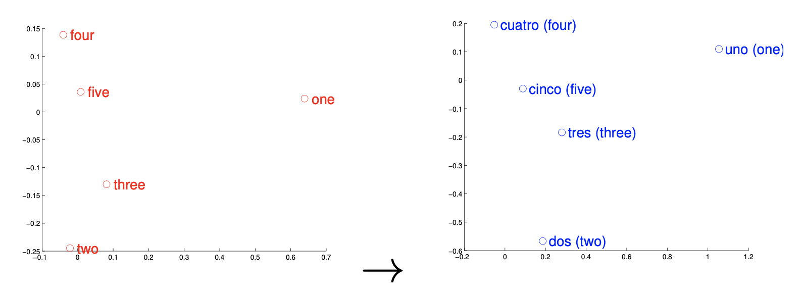
FIGURE 2.4: Representations of numbers in English and Spanish (Source: Mikolov, Le, and Sutskever (2013)).

This technique was then used for other experiments. One use case is the detection of dictionary errors. Taking translations from a dictionary and computing their geometric distance returns a confidence measure. Closely evaluating the translations with low confidence and outputting an alternative (one that is closest in vector space) results in a plain way to assess dictionary translations. Furthermore, training the word embeddings on a large corpora makes it possible to give sensible out-of-dictionary predictions for words. This was tested by randomly removing a part of the vocabulary before. Taking a look at the predictions revealed that they were often to some extent related to the translations with regard to meaning and semantics. Despite the accomplishments in other tasks, translations between distant languages exposed shortcomings of word embeddings. For example, the accuracy for translations between English and Vietnamese seemed significantly lower. This can be ascribed to both languages not having a good one-to-one correspondence because the concept of a word is different than in English. In addition, the used Vietnamese model contains numerous synonyms, which complicates making exact predictions (see Mikolov, Le, and Sutskever (2013)).

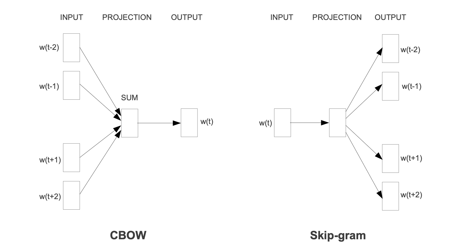
Turning the attention to one of the most impactful embedding techniques, word2vec. It was proposed by Mikolov, Chen, et al. (2013 a) and is not a singular algorithm. It can rather be seen as a family of model architectures and optimizations to learn word representations. Word2vec’s popularity also stems from its success on multiple downstream natural language processing tasks. It has a very simple structure which is based on a basic feed forward neural network. They published multiple papers (see Mikolov, Chen, et al. (2013 a)], Mikolov, Le, and Sutskever (2013), Mikolov, Sutskever, et al. (2013)) that are stemming around two different but related methods for learning word embeddings (see Figure 2.5). Firstly, the Continuous bag-of-words model aims to predict the middle word based on surrounding context words. Hence, it considers components before and after the target word. As the order of words in the context is not relevant, it is called a bag-of-words model. Secondly, the Continuous skip-gram model only considers the current word and predicts others within a range before and after it in the same sentence. Both of the models use a softmax classifier for the output layer.

FIGURE 2.5: CBOW and Skip-gram architecture (Source: Mikolov, Chen, et al. (2013 a)).

Then, Bojanowski et al. (2016) built on skip-gram models by accounting for the morphology (internal structure) of words. A different classical embedding architecture that has to be at least mentioned is the GloVe model, which does not use a neural network but incorporates local context information with global co-occurrence statistics.

2.1.3 Encoder-Decoder

The field of natural language processing is concerned with a variety of different tasks surrounding text. Depending on the type of NLP problem, the network may be confronted with variable length sequences as input and/or output. This is the case for many compelling applications, such as question answering, dialogue systems or machine translation. In the following, many examples will explore machine translations in more detail, since it is a major problem domain. Regarding translation tasks, it becomes obvious that input sequences need to be mapped to output sequences of different lengths. To manage this type of input and output, a design with two main parts could be useful. The first one is called the encoder because, in this part of the network, a variable length input sequence is transformed into a fixed state. Next, the second component called the decoder maps the encoded state to an output of a variable length sequence. As a whole, it is known as an encoder-decoder or sequence-to-sequence architecture and has become an effective and standard approach for many applications which even recurrent neural networks with gated hidden units have trouble solving successfully. Deep RNNs may have a chance, but different architectures like encoder-decoder have proven to be the most effective. It can even deal with different word orders and active, as well as passive voice (Sutskever, Vinyals, and Le 2014). A simplified example of the encoder-decoder model can be seen in 2.6.

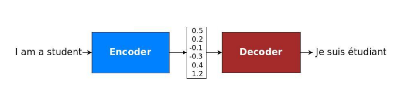
FIGURE 2.6: Translation through simplified seq2seq model (Source: Manning, Goldie, and Hewitt (2022)).

Before going through the equations quantifying the concepts, it makes sense to examine the sequence-to-sequence design proposed by Cho et al. (2014). An encoder-RNN processes the input sequence of length $n_x$ and computes a fixed-length context vector $C$, which is usually the final hidden state of the encoder or a simple function of the hidden states. After the input sequence is processed, it is added to the hidden state and passed forward in time through the recurrent connections between the hidden states in the encoder. Despite the context vector usually being a simple function of the last hidden state, its role cannot be underestimated. Specifically, the encoded state summarizes important information from the input sequence, e.g. the intent in a question answering task or the meaning of a text in the case of machine translation. After the context is passed to every hidden state of the decoder, the decoder RNN uses this information to produce the target sequence of length $n_y$, which can of course vary from $n_x$.

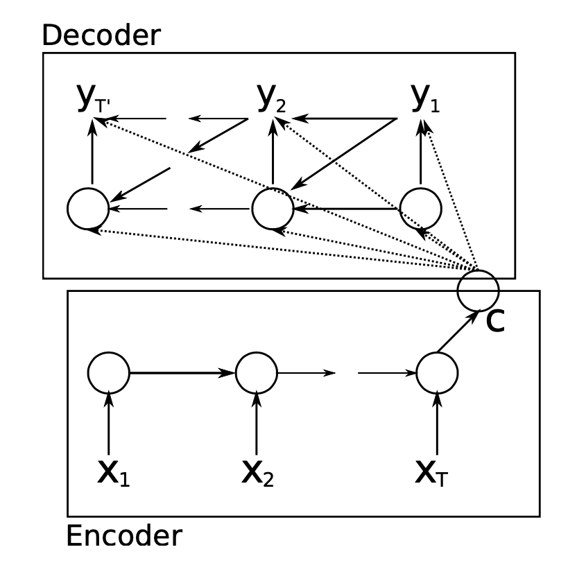
FIGURE 2.7: Encoder-decoder architecture (Source: Cho et al. (2014)).

At the latest through the above illustration, it is clear that the decoder is particularly interesting to look at in the form of equations. The notation mainly follows Cho et al. (2014). The decoder is another type of RNN which is trained to predict the target based on the hidden state at the last time step. However, unlike regular RNNs, it is also conditioned on the output of the last time step ($y_{t-1}$) and a summary of the input c. Therefore, the hidden state of the decoder is computed by:

\[h_d^{[t]} = f(h_d^{[t-1]},y^{[t-1]},c). \label{eqn:h_dec}\]

Similarly, each conditional probability is given by the following, where $f$ is a non-linear activation function (and must produce probabilities in , e.g. the softmax function):

\[P(y^{[t]}|y^{[1]}, \dots ,y^{[t-1]},c) = f(h_d^{[t]}, y^{[t-1]}, c). \label{eqn:P_dec}\]

The two parts are jointly trained to maximize the conditional log-likelihood, where $\theta$ denotes the set of model parameters and $(x_n, y_n)$ is an (input sequence, output sequence) pair from the training set with size $N$:

\[\max_\theta \frac{1}{N} \displaystyle \sum_{n=1}^{N} \log p_{\theta}(y_n|x_n). \label{eqn:train_dec}\]

The best probability is usually found by using the beam search algorithm. The core idea of it is that on each step of the decoder, we keep track of the $k$ most probable partial translations (which are called hypotheses).

Examining the translation presented in with hidden units unrolled through time could look like in 2.8. In particular, multiple hidden layers are recommended by the researchers. The idea is that lower layers compute lower-level features and higher layers compute higher-level features.

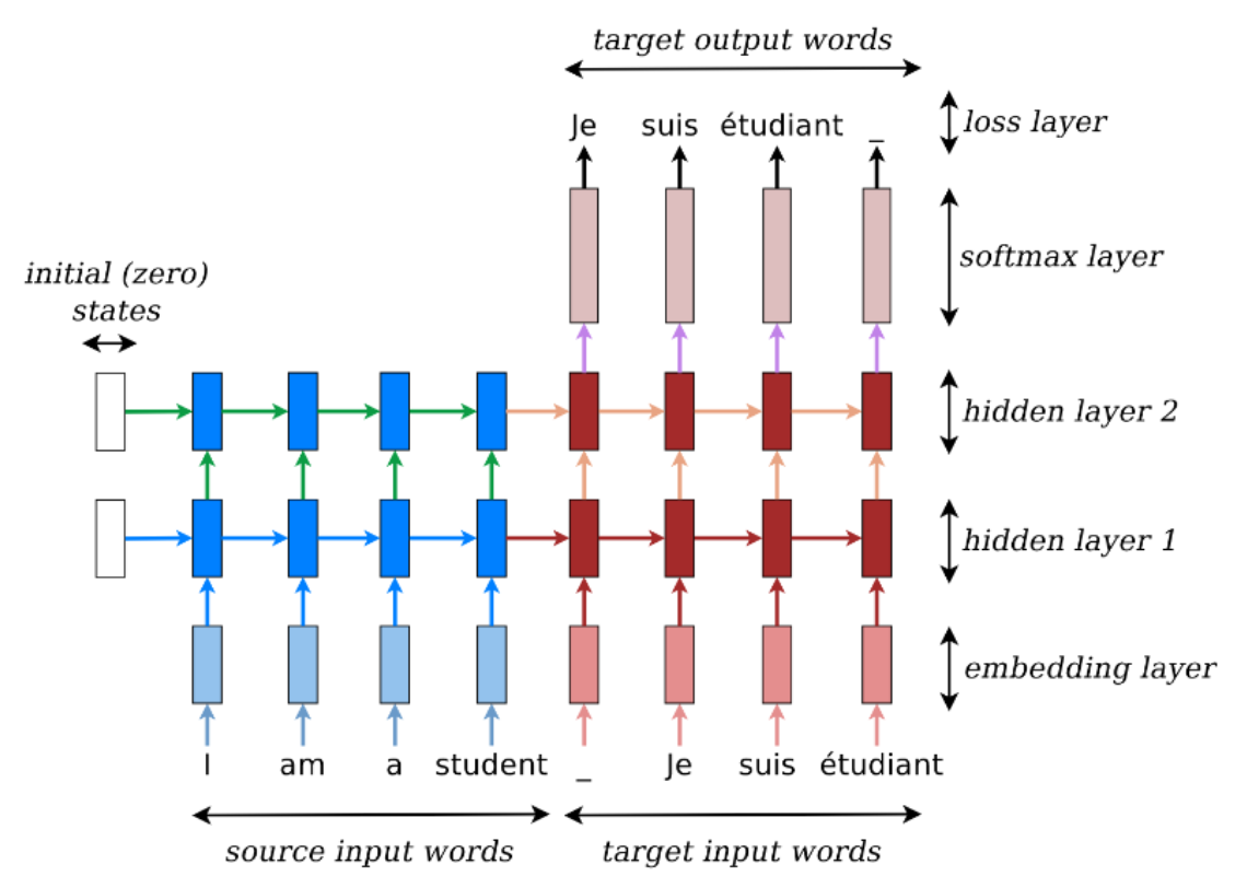
FIGURE 2.8: Translation through seq2seq model (Source: Manning, Goldie, and Hewitt (2022)).

Gated recurrent networks, especially long short-term memory networks, have been found to be effective in both components of the sequence-to-sequence architecture. Furthermore, it was revealed that deep LSTMs significantly outperform shallow LSTMs. Each additional layer reduced perplexity by nearly 10%, possibly due to their much larger hidden state. For example, Sutskever, Vinyals, and Le (2014) used deep LSTMs with 4 layers and 1000 cells at each layer for 1000-dimensional word embeddings. Thus, in total, 8000 real numbers are used to represent a sentence. For simplification, the neural networks are in the following referred to as RNNs which is not contradicting the insights of this paragraph as LSTMs are a type of gated RNNS (Sutskever, Vinyals, and Le 2014).

2.1.4 Attention

Although encoder-decoder architectures simplified dealing with variable length sequences, they also caused complications. Due to their design, the encoding of the source sentence is a single vector representation (context vector). The problem is that this state must compress all information about the source sentence in a single vector and is commonly referred to as the bottleneck problem. To be precise, the entire semantics of arbitrarily long sentences need to be wrapped into a single hidden state. Moreover, it constitutes a different learning problem because the information needs to be passed between numerous time steps. This leads to vanishing gradients within the network as a consequence of factors less than 1 multiplied with each other at every point. To illustrate, the last sentence is an ideal example of one in which an encoder-decoder approach could have difficulty coping. In particular, if the sentences are longer than the ones in the training corpus (Manning, Goldie, and Hewitt 2022).

Due to the aforementioned reasons, an extension to the sequence-to-sequence architecture was proposed by Bahdanau, Cho, and Bengio (2014), which learns to align and translate jointly. For every generated word, the model scans through some positions in the source sentence where the most relevant information is located. Afterwards, based on the context around and the previously generated words, the model predicts the target word for the current time step. This approach is called attention, as it emulates human-like (cognitive) attention. As a result of directly looking at the source and bypassing the bottleneck, it provides a solution to the problem. Then, it mitigates the vanishing gradient problem, since there is now a shortcut to faraway states. Consequently, incorporating the attention mechanism has been shown to considerably boost the performance of models on NLP tasks.

A walkthrough of the example below should resolve any outstanding questions regarding the procedure of the attention mechanism. The source sentence is seen on the bottom left, which is given in French and acts as the input for the encoder-RNN (in red). Then, the attention scores (in blue) are computed by taking the dot product between the previous output word and input words. Next, the softmax function turns the scores into a probability distribution (in pink). They are used to take a weighted sum of the encoder’s hidden states and form the attention output, which mostly contains information from the hidden states that received high attention. Afterwards, the attention output is concatenated with the decoder hidden state (in green), which is applied to compute the decoder output as before. In some scenarios, the attention output is also fed into the decoder (along with the usual decoder input). This specific example was chosen because "entarter" means "to hit someone with a pie" and is therefore a word that needs to be translated with many words. As a consequence of no existing direct equivalents for this phrase, it is expected that there is not only one nearly non-zero score. In this snapshot, the attention distribution can be seen to have two significant contributors.

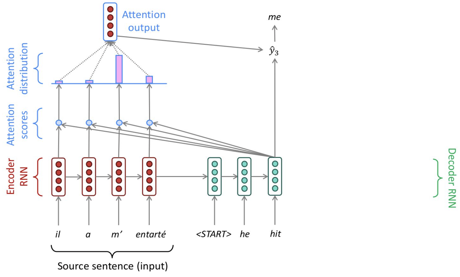
FIGURE 2.9: Translation process with attention mechanism (Source: Manning, Goldie, and Hewitt (2022)).

The following equations aim to compactly represent the relations brought forward in the last paragraphs and mainly follow Manning, Goldie, and Hewitt (2022). The attention scores $e^{[t]}$ are computed by scalarly combining the hidden state of the decoder with all of the hidden states of the encoder:

\[e^{[t]} = [(h_{d}^{[t]})^T h_{e}^{[1]}, \ldots , (h_{d}^{[t]})^T h_{e}^{[N]} ].\]

Besides the basic dot-product attention, there are also other ways to calculate the attention scores, e.g. through multiplicative or additive attention. Although they will not be further discussed at this point, it makes sense to at least mention them. Then, applying the softmax to the scalar scores results in the attention distribution $\alpha^{[t]}$, a probability distribution whose values sum up to 1:

\[\alpha^{[t]} = softmax(e^{[t]}).\]

Next, the attention output $a^{[t]}$ is obtained by the attention distribution acting as a weight for the encoder hidden states:

\[a^{[t]} = \sum_{i=1}^{N} \alpha_i^{[t]} h_{e,i}.\]

Concatenating attention output with decoder hidden state and proceeding as in the non-attention sequence-to-sequence model are the final steps:

\[o^{[t]} = f(a^{[t]} h_d^{[t]}).\]

By visualizing the attention distribution, also called alignments (see Bahdanau, Cho, and Bengio (2014)), it is easy to observe what the decoder was focusing on and understand why it chose a specific translation. The x-axis of the plot of below corresponds to the words in the source sentence (English) and the y-axis to the words in the generated translation (French). Each pixel shows the weight of the source word for the respective target word in grayscale, where 0 is black and 1 is white. As a result, which positions in the source sentence were more relevant when generating the target word becomes apparent. As expected, the alignment between English and French is largely monotonic, as the pixels are brighter, and therefore the weights are higher along the main diagonal of the matrix. However, there is an exception because adjectives and nouns are typically ordered differently between the two languages. Thus, the model (correctly) translated "European Economic Area" into "zone économique européene". By jumping over two words ("European" and "Economic"), it aligned "zone" with "area". Then, it looked one word back twice to perfect the phrase "zone économique européene". Additional qualitative analysis has shown that the model alignments are predominantly analogous to our intuition.

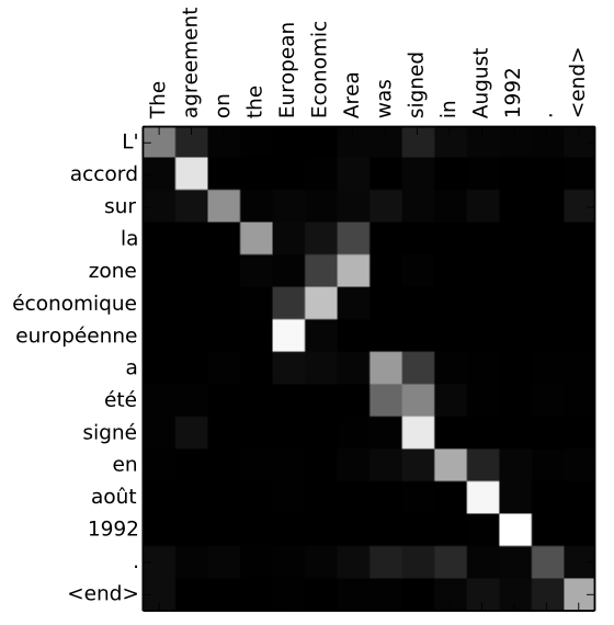
FIGURE 2.10: Attention alignments (Source: Bahdanau, Cho, and Bengio (2014)).

2.1.5 Transformer

For this section, Manning, Goldie, and Hewitt (2022) constitutes the main source.

RNNs are unrolled from one side to the other. Thus, from left to right and right to left. This encodes linear locality, which is a useful heuristic because nearby words often affect each other’s meaning. But how is it when distant words need to interact with each other? For instance, if we mention a person at the beginning of a text portion and refer back to them only at the very end, the whole text in between needs to be tracked back (see below). Hence, RNNs take $O(\text{sequence length})$ steps for distant word pairs to interact. Due to gradient problems, it is therefore hard to learn long-distance dependencies. In addition, the linear order is ingrained. Even though, as known, the sequential structure does not tell the whole story.

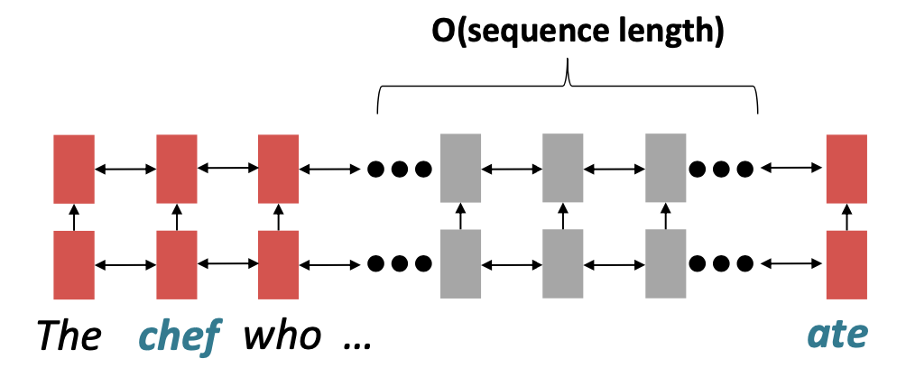
FIGURE 2.11: Sequential processing of recurrent model (Source: Manning, Goldie, and Hewitt (2022)).

GPUs can perform multiple calculations simultaneously and could help to reduce the execution time of the deep learning algorithm massively. However, forward and backward passes lack parallelizability in recurrent models and have $O(\text{sequence length})$. To be precise, future hidden states cannot be computed in full before past states have been computed. This inhibits training on massive data sets. indicates the minimum number of steps before the respective state can be calculated.

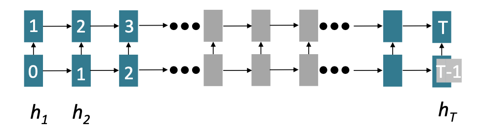
FIGURE 2.12: Sequential processing of recurrent model with number of steps indicated (Source: Manning, Goldie, and Hewitt (2022)).

After proving that attention dramatically increases performance, google researchers took it further and based transformers solely on attention, so without any RNNs. For this reason, the paper in which they were introduced is called "Attention is all you need". Spoiler: It is not quite all we need, but more about that on the following pages. Transformers have achieved great results on multiple settings such as machine translation and document generation. Their parallelizability allows for efficient pretraining and leads them to be the standard model architecture. In fact, all top models on the popular aggregate benchmark GLUE are pretrained and Transformer-based. Moreover, they have even shown promise outside of NLP, e.g. in Image Classification, Protein Folding and ML for Systems (see Dosovitskiy, Beyer, Kolesnikov, Weissenborn, Zhai, Unterthiner, Dehghani, Minderer, Heigold, Gelly, and others (2020), Jumper et al. (2021), Zhou et al. (2020), respectively).

If recurrence has its flaws, another adjustment of the attention mechanism might be beneficial. Until now, it was defined from decoder to encoder. Alternatively, attention could also be from one state to all states in the same set. This is the definition of self-attention, which is encoder-encoder or decoder-decoder attention (instead of encoder-decoder) and represents a cornerstone of the transformer architecture. depicts this process in which each word attends to all words in the previous layer. Even though in practice, most arrows are omitted eventually.

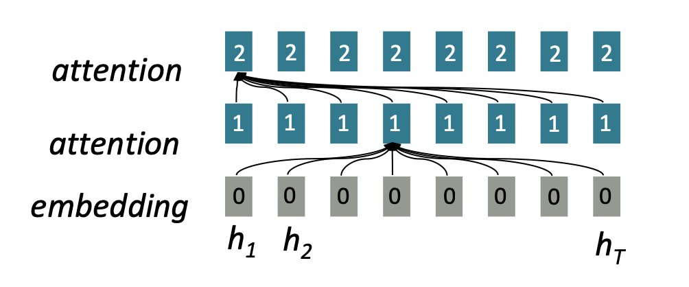
FIGURE 2.13: Connections of classic attention mechanism (Source: Manning, Goldie, and Hewitt (2022)).

Thinking of self-attention as an approximate hash table eases understanding its intuition. To look up a value, queries are compared against keys in a table. In a hash table, which is shown on the left side of , there is exactly one key-value pair for each query (hash). In contrast, in self-attention, each key is matched to varying degrees by each query. Thus, a sum of values weighted by the query-key match is returned.

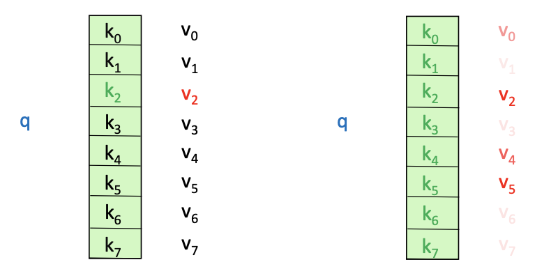
FIGURE 2.14: Comparison of classic attention mechanism with self-attention with hash tables (Source: Manning, Goldie, and Hewitt (2022)).

The process briefly described in the last paragraph can be summarized by the following steps that mainly follow Manning, Goldie, and Hewitt (2022). Firstly, deriving query, key, and value for each word $x_i$ is necessary: \[q_i = W^Q x_i , \hspace{3mm} k_i = W^K x_i, \hspace{3mm} v_i = W^V x_i\]

Secondly, the attention scores have to be calculated:

\[e_{ij} = q_i k_j\]

Thirdly, to normalize the attention scores, the softmax function is applied:

\[\alpha_{ij} = softmax( e_{ij} ) = \frac{exp(e_{ij})}{\displaystyle \sum_k e_{ij}}\]

Lastly, taking the weighted sum of the values results in obtaining the attention output:

\[a_{i} = \displaystyle \sum_j \alpha_{ij} v_j\]

Multiple advantages of incorporating self-attention instead of recurrences have been revealed. Since all words interact at every layer, the maximum interaction distance is $O(1)$ and is a crucial upgrade. In addition, the model is deeply bidirectional because each word attends to the context in both directions. As a result of these advances, all word representations per layer can be computed in parallel. Nevertheless, some issues have to be discussed. Attention does no more than weighted averaging. So without neural networks, there are no element-wise non-linearities. Their importance cannot be understated and shows why attention is not actually all that is needed. Furthermore, bidirectionality is not always desired. In language modelling, the model should specifically be not allowed to simply look ahead and observe more than the objective allows. Moreover, the word order is no longer encoder, and it is bag-of-words once again.

Fortunately, the previously mentioned weaknesses have been addressed for the original transformer-architecture proposed by Vaswani, Shazeer, Parmar, Uszkoreit, Jones, Gomez, et al. (2017 a). The first problem can be easily fixed by applying a feed forward layer to the output of attention. It provides non-linear activation as well as extra expressive power. Then, for cases in which bidirectionality contradicts the learning objective, future states can be masked so that attention is restricted to previous states. Moreover, the loss of the word can be corrected by adding position representations to the inputs.

The more complex deep learning models are, the closer they become to model the complexity of the real world. That is why the transformer encoder and decoder consist of many layers of self-attention with a feed forward network, which is necessary to extract both syntactic and semantic features from sentences. Otherwise, using word embeddings, which are semantically deep representations between words, would be unnecessary (Sejnowski 2020). At the same time, training deep networks can be troublesome. Therefore, some tricks are applied to help with the training process.

One of them is to pass the "raw" embeddings directly to the next layer, which prevents forgetting or misrepresent important information as it is passed through many layers. This process is called residual connections and is also believed to smoothen the loss landscape. Additionally, it is problematic to train the parameters of a given layer when its inputs keep shifting because of layers beneath. Reducing uninformative variation by normalizing within each layer to mean zero and standard deviation to one weakens this effect. Another challenge is caused by the dot product tending to take on extreme values because of the variance scaling with increasing dimensionality $d_k$. It is solved by Scaled Dot Product Attention (see Figure 2.15), which consists of computing the dot products of the query with its keys, dividing them by the dimension of keys $\sqrt{d_k}$, and applying the softmax function next to receive the weights of the values.

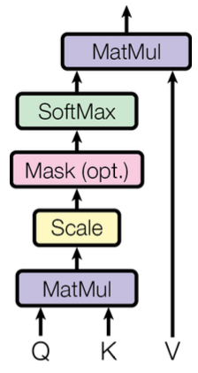
FIGURE 2.15: Scaled dot-product attention (Source: Vaswani, Shazeer, Parmar, Uszkoreit, Jones, Gomez, et al. (2017 a)).

Attention learns where to search for relevant information. Surely, attending to different types of information in a sentence at once delivers even more promising results. To implement this, the idea is to have multiple attention heads per layer. While one attention head might learn to attend to tense information, another might learn to attend to relevant topics. Thus, each head focuses on separate features, and construct value vectors differently. Multi-headed self-attention is implemented by simply creating $n$ independent attention mechanisms and combining their outputs.

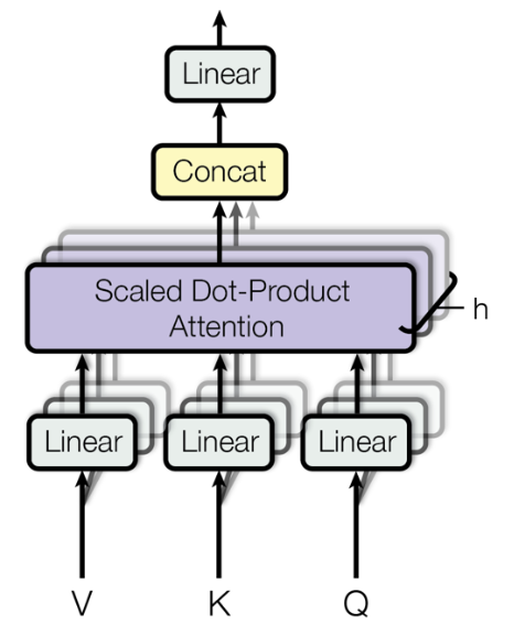
FIGURE 2.16: Multi-head attention (Source: Vaswani, Shazeer, Parmar, Uszkoreit, Jones, Gomez, et al. (2017 a)).

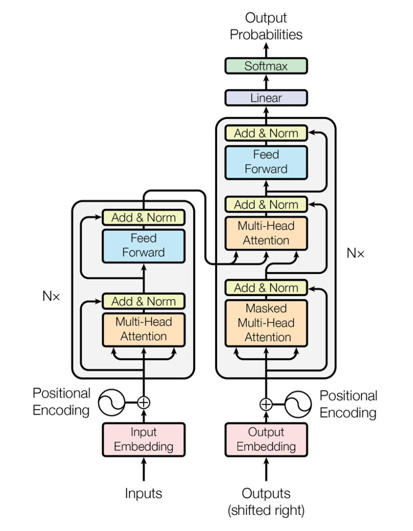
At this point, every part that constitutes the encoder in the transformer architecture has been introduced (see Figure 2.17). First, positional encodings are included in the input embeddings. There are multiple options to realize this step, e.g. through sinusoids. The multi-head attention follows, which was just mentioned. "Add & Norm" stands for the residual connections and the normalization layer. A feed forward network follows, which is also accompanied by residual connections and a normalization layer. All of it is repeated $n$ times. For the decoder, the individual components are similar. One difference is that the outputs go through masked multi-head attention before multi-head attention and the feed forward network (with residual connections and layer normalization). It is critical to ensure that the decoder cannot peek at the future. To execute this, the set of keys and queries could be modified at every time step to only include past words. However, it would be very inefficient. Instead, to enable parallelization, future states are masked by setting the attention scores to $-\infty$. After the decoder process is also repeated $n$ times, a linear layer is added to project the embeddings into a larger vector that has the length of the vocabulary size. At last, a softmax layer generates a probability distribution over the possible words.

FIGURE 2.17: Transformer architecture (Source: Vaswani, Shazeer, Parmar, Uszkoreit, Jones, Gomez, et al. (2017 a)).

2.1.6 Transformer architectures: BERT, T5, GPT-3

"You shall know a word by the company it keeps", an adage by linguist John Rupert Firth from 1957 goes. Even earlier, in 1935, he stated that "... the complete meaning of a word is always contextual, and no study of meaning apart from a complete context can be taken seriously". The quotes of the famous linguist sum up the motivation to learn word meaning and context perfectly. Many years later, in 2017, pretraining word embeddings started. However, some complications arise from solely pretraining the first part of the network. For instance, to teach the model all contextual aspects of language, the training data for the downstream task (e.g. question answering) needs to be adequate. Additionally, most of the parameters are usually randomly initialized. presents the network discussed, in which the word "movie" gets the same embedding irrespective of the sentence it appears in. On the contrary, parameters in modern NLP architectures are initialized via pretraining (see Figure 2.18). Furthermore, during the pretraining, certain input parts are hidden to train the model to reconstruct them. This leads to building suitable parameter initializations and robust probability distributions over language.

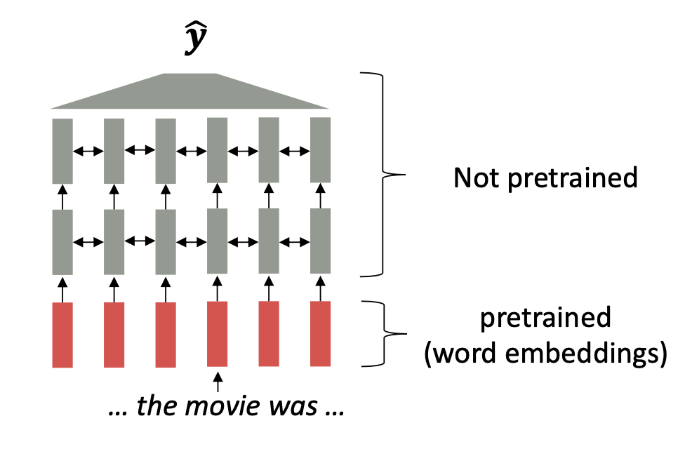
FIGURE 2.18: Partly pre-trained model (Source: Manning, Goldie, and Hewitt (2022)).

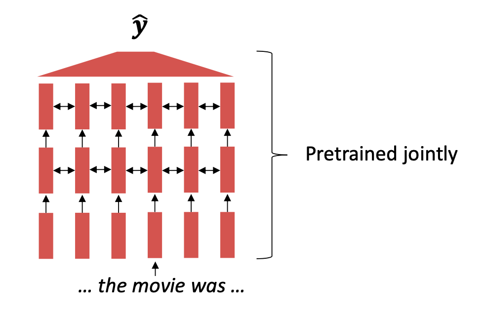
FIGURE 2.19: Jointly pre-trained model (Source: Manning, Goldie, and Hewitt (2022)).

Classic machine learning does not match human learning. Specifically referring to training a model from scratch, and only being able to learn from the training data. In contrast, human beings already have prior knowledge they can apply to new tasks. Transfer learning emulates this by using an already trained network. The main idea is to use a model that was pretrained on a hard, general language understanding task using endless amounts of data, so that, it eventually contains the best possible approximation of language understanding. Afterwards, the training data for the new task is applied to slightly modify the weights of the pretrained model, which is referred to as fine-tuning (Manning, Goldie, and Hewitt 2022).

The specific architecture of a transformer model affects the type of pre-training, and favourable use cases. In the following, three different but very influential transformer architectures will be discussed. BERT can be seen as stacked encoders (Devlin et al. 2018 b), T5 aims to combine the good parts of encoders and decoders (Raffel et al. 2019 a), while GPT are stacked decoders (Brown et al. 2020).

2.1.6.1 BERT

Transfer learning led to state-of-the-art results in natural language processing. One of the architectures that led the way was BERT, which stands for Bidirectional Encoder Representations from Transformers. It receives bidirectional context, which is why it is not a natural fit for language modelling. To train it on this objective regardless, masked language modelling was proposed. The main idea is to cover up a fraction of the input words and let the model predict them. In this way, the LM objective can be used while sustaining connections to words in the future. The masked LM for BERT randomly predicts 15% of all word tokens in each sequence. Of those, 80% are replaced by the \[MASK\] token, 10% by a random token, and 10% remain unchanged. Moreover, because the masked words are not even seen in the fine-tuning phase, the model cannot get complacent and relies on strong representations of non-masked words. Initially, BERT had an additional objective of whether one sentence follows another, which is known as next sentence prediction. However, it was dropped in later work due to having an insignificant effect.

BERT is hugely versatile and was greatly popular after its release. Fine-tuning BERT led to outstanding results on a variety of applications, including question answering, sentiment analysis and text summarization. Thanks to its design, if the task involves generating sequences, pretrained decoders outperform pretrained encoders like BERT. Even though, it would not be recommended for autoregressive generation, up to this day, "small" models like BERT are applied as general tools for numerous tasks.

2.1.6.2 T5

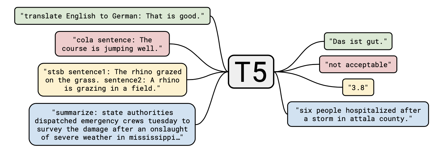
The Text-To-Text Transfer Transformer (T5) is a new model that can be regarded as an application of the insights gathered by an extensive empirical study searching for the best transfer learning techniques. It is pretrained on Colossal Clean Crawled Corpus (C4), an open-source dataset. Raffel et al. (2019 a) found that the best pretraining objective to use for the encoder component was span corruption. In short, different length word groups (spans) are replaced with unique placeholders, and let the model decode them. Text preprocessing is necessary for its implementation. For the decoder, it is still a language modelling task. Compared to models like BERT, which can only output a span of the input or a class label, T5 reframes all NLP tasks into a unified text-to-text format, where inputs and outputs always consist of text strings. As a result, the same model, loss function, and hyperparameters can be used on any NLP task, such as machine translation, document summarization, question answering, and classification tasks like sentiment analysis. T5 can even be applied to regression tasks by training it to predict the string representation of a number (and not the number itself). Examples of potential use cases are depicted in below.

FIGURE 2.20: Applications of T5 model (Source: Raffel et al. (2019 a)).

2.1.6.3 GPT-3

As previously stated, the neural architecture influences the type of pretraining. The original GPT architecture consists of a Transformer decoder with 12 layers (Radford et al. 2018). For decoders, it is sensible to simply pretrain them as language models. Afterwards, they can be used as generators to fine-tune their probability of predicting the next word conditioned on the previous words. The models are suitable for tasks similar to the training, including any type of dialogue and document summarization. Transformer language models are great for transfer learning. They are fine-tuned by randomly initializing a softmax classifier on top of the pretrained model and training both (with only a very small learning rate and a small number of epochs) so that the gradient propagates through the whole network.

The success of BERT in 2018 prompted a "gold rush" in NLP, in which ever greater language models were created. One that topped the headlines and used a customer supercluster for computation was the third iteration of the GPT architecture by OpenAI, known as GPT-3. reveals why GPT-3 is a famous example of current research focusing on scaling up neural language models. While the largest T5 model has 11 billion parameters, GPT-3 has 175 billion parameters. Moreover, the training data set contains around 500 billion tokens of text, while the average young american child hears around 6 million words per year (Hart and Risley 1995). The results of huge language models suggest that they perform some form of learning (without gradient steps) simply from examples provided via context. The tasks are specified by the in-context examples, and the conditional probability distribution simulates performing the task to an extent.

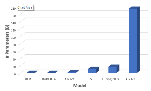
FIGURE 2.21: Comparison of number of parameters between Transformer-architectures (Source: Saifee (2020)).

2.1.7 Current Topics

2.1.7.1 Concerns regarding growing size of Language Models

As the last chapter ended with GPT-3 and emphasized the concerning trend of ever larger language models, one could ask which other costs arise from the developments. Risks and harms among environmental and financial costs have been studied by Bender et al. (2021). They state that marginalized communities are not only less likely to benefit from LM progress, but also more likely to suffer from the environmental repercussions of increasing resource consumption. Strubell, Ganesh, and McCallum (2019 a) estimated that training a Transformer (big) model resulted in 249t of $CO_2$. To compare, an average human is responsible for approximately 5t of $CO_2$ per year (Ritchie, Roser, and Rosado 2020). In addition, they discovered that an estimated increase of 0.1 in BLEU score increased computation costs by $ 150,000 (for English to German translations). Furthermore, larger models require more data to sufficiently train them. This has resulted in large but poorly documented training data sets. Multiple risks can be mitigated if there is a common understanding of the model’s learnings.

Moreover, it has been argued that datasets consisting of web data over-represent hegemonic views and encode bias towards marginalized communities. This is among other factors due to internet access being unevenly distributed. In particular, there is an over-representation of younger internet users and those from developed countries. It is generally naive to educate AI systems on all aspects of the complex world, and hope for the beautiful to prevail (Bender et al. 2021).

2.1.7.2 Improving Understanding of Transformer-based models

The results of transformer-based models clearly show that they deliver successful results. However, it is less clear why. The size of the models makes it difficult to experiment with them. Nevertheless, having a limited understanding restrains researchers from coming up with further improvements. Therefore, multiple papers analysed BERT’s attention in search of an improved understanding of large transformer models. BERT is a smaller model out of the more popular ones, and its attention is naturally interpretable because the attention weight indicates how significant a word is for the next representation of the current word (Clark et al. 2019). In the following, some of the findings are going to be shared.

BERT representations are rather hierarchical than linear, and they include information about parts of speech, syntactic chunks and roles (Lin, Tan, and Frank 2019, @Liu2019) Furthermore, it has semantic knowledge. For example, BERT can recognize e.g. that "to tip a chef" is better than "to tip a robin" but worse than "to tip a waiter" ((Ettinger 2019)). However, it makes sense that BERT has issues with knowledge that is assumed and not mentioned, which especially refers to visual and perceptual properties (Da and Kasai 2019). Additionally, BERT struggles with inferences, e.g. even though it is known that "people walk into houses" and "houses are big", it cannot infer that "houses are bigger than people" (Forbes, Holtzman, and Choi 2019).

While it is true that different transformer heads attend to various patterns (see ), interestingly, most of them could be neglected without notable performance loss (Voita et al. 2019). Probing attention maps can be tedious, but allows to gain knowledge of common patterns, such as an unexpected amount focusing on the delimiter token \[SEP\].

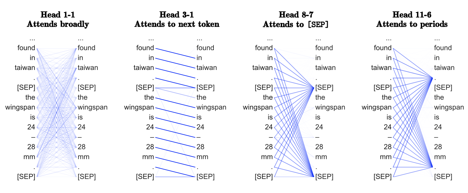
FIGURE 2.22: Common patterns of attention heads (Source: Clark et al. (2019)).

2.1.7.3 Few-Shot Learning

For NLP tasks, the model is usually trained on a set of labelled examples and is expected to generalize to unseen data. Annotating is not only costly but also difficult to gather for numerous languages, domains, and tasks. In practice, there is often only a very limited amount of labelled examples. Consequently, few-shot learning is a highly relevant research area (Schick and Schütze 2020). It defines a model that is trained on a limited number of demonstrations to guide its predictions. Referring back to , the benefits of lower computational and environmental costs have to be mentioned.

Traditional fine-tuning uses a large corpus of example tasks, and the model is updated repeatedly with gradient steps so that it adapts to the task with minimal accuracy error.

In contrast, few-shot applications have to complete tasks at test time with only forward passes. They have three main parts: the task description, examples, and the prompt. In Figure ??, the task is a translation from English to French, a few examples, as well as the word that should be translated are given. Moreover, zero-shot and one-shot learning refer to the model predicting with no and one learned example, respectively (Brown et al. 2020).

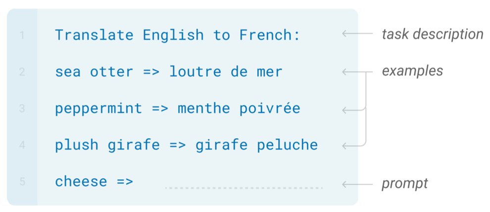
FIGURE 2.23: Few-shot learning (Source: Brown et al. (2020)).

It is complicated to create the few-shot examples, since the application relies on them to express the task. This is why smaller models are susceptible to examples written unfavourably. In Brown et al. (2020), it was shown that few-shot performance scales with the number of model parameters. Even though GPT-3’s in-context learning improved few-shot prompting capabilities, it is still sensitive to the order of training examples, decoding strategy, and hyperparameter selection. All of this combined with the fact that current research uses larger or held-out data sets leads to the suspicion that the true few-shot ability of language models is overestimated (Perez, Kiela, and Cho 2021 a).

Moreover, Lialin et al. (2022) have found that common transformer models could not resolve compositional questions in a zero-shot fashion and that the model’s parameter count does not correlate with performance. This indicates a limitation for zero-shot prompting with the existing pre-training objectives. However, different models provided the best accuracy with regard to different symbolic reasoning tasks. This suggests that optimization or masking strategies could be more significant than the pre-training, data set size or model architecture.

2.1.8 Summary

Natural Language Processing has been one of the most exciting fields of machine learning in the last decade considering all the breakthroughs discussed in this work. Word embeddings made it possible and allowed developers to encode words as dense vectors that capture their underlying semantic content. In this way, similar words are embedded close to each other in a lower-dimensional feature space. Another important challenge was solved by encoder-decoder (also called sequence-to-sequence) architectures, which made it possible to map input sequences to output sequences of different lengths. They are especially useful for complex tasks like machine translation, video captioning or question answering. A significant state-of-the-art technique is attention, which enabled models to actively shift their focus – just like humans do. It allows following one thought at a time while suppressing information irrelevant to the task. As a consequence, it has been shown to significantly improve performance for tasks like machine translation. By giving the decoder access to directly look at the source, the bottleneck is avoided and at the same time, it provides a shortcut to faraway states and thus helps with the vanishing gradient problem. One of the most recent data modelling techniques is the transformer, which is solely based on attention and does not have to process the input data sequentially. Therefore, the deep learning model is better in remembering context-induced earlier in long sequences. It is the dominant paradigm in NLP currently and makes better use of GPUs because it can perform parallel operations. Transformer architectures like BERT, T5 or GPT-3 are pre-trained on a large corpus and can be fine-tuned for specific language tasks. They can generate stories, poems, code and much more. Currently, there seems to be breaking transformer news nearly every week with no sign of slowing. This is why many trends could be recognized as relevant current topics. One of them is increasing concerns regarding the growing size of language models and the correlated environmental and financial costs. Another active research aspect is concerned with improving the understanding of transformer-based models to further advance them. Additionally, there are many studies about achieving respectable results on language modelling tasks after only learning from a few examples, which is known as few-shot learning.

2.2 State-of-the-art in Computer Vision

Author: Vladana Djakovic

Supervisor: Daniel Schalk

2.2.1 History

The first research about visual perception comes from neurophysiological research performed in the 1950s and 1960s on cats. The researchers used cats as a model to understand how human vision is compounded. Scientists concluded that human vision is hierarchical and neurons detect simple features like edges followed by more complex features like shapes and even more complex visual representations. Inspired by this knowledge, computer scientists focused on recreating human neurological structures.

At around the same time, as computers became more advanced, computer scientists worked on imitating human neurons’ behavior and simulating a hypothetical neural network. In his book “The Organization of Behaviour” (1949) Donald Hebbian stated that neural pathways strengthen over each successive use, especially between neurons that tend to fire at the same time, thus beginning the long journey towards quantifying the complex processes of the brain. The first Hebbian network, inspired by this neurological research, was successfully implemented at MIT in 1954 (Jaspreet 2019).

New findings led to the establishment of the field of artificial intelligence in 1956 on-campus at Dartmouth College. Scientists began to develop ideas and research how to create techniques that would imitate the human eye.

In 1959 early research on developing neural networks was performed at Stanford University, where models called “ADALINE” and “MADALINE,” (Multiple ADAptive LINear Elements) were developed. Those models aimed to recognize binary patterns and could predict the next bit (“Neural Networks - History” 2022).

Starting optimism about Computer Vision and neural networks disappeared after 1969 and the publication of the book “Perceptrons” by Marvin Minsky, founder of the MIT AI Lab, stated that the single perception approach to neural networks could not be translated effectively into multi-layered neural networks. The period that followed was known as AI Winter, which lasted until 2010, when the technological development of computer and the internet became widely used. In 2012 breakthroughs in Computer Vision happened at the ImageNet Large Scale Visual Recognition Challenge (ILSVEC). The team from the University of Toronto issued a deep neural network called AlexNet (Krizhevsky, Sutskever, and Hinton 2012 a) that changed the field of artificial intelligent and Computer Vision (CV). AlexNet achieved an error rate of 16.4%.

From then until today, Computer Vision has been one of the fastest developing fields. Researchers are competing to develop a model that would be the most similar to the human eye and help humans in their everyday life. In this chapter the author will describe only a few recent state-of-the-art models.

2.2.2 Supervised and unsupervised learning

As part of artificial intelligence (AI) and machine learning (ML), there are two basic approaches:

supervised learning;
unsupervised learning.

Supervised learning (Education 2020 a) is used to train algorithms on labeled datasets that accurately classify data or predict outcomes. With labeled data, the model can measure its accuracy and learn over time. Among others, we can distinguish between two common supervised learning problems:

classification,
regression.

In unsupervised learning (Education 2020 b), unlabelled datasets are analyzed and clustered using machine learning algorithms. These algorithms aim to discover hidden patterns or data groupings without previous human intervention. The ability to find similarities and differences in information is mainly used for three main tasks:

clustering,
association,
dimensionality reduction.

Solving the problems where the dataset can be both labeled and unlabeled requires a semi-supervised approach that lies between supervised and unsupervised learning. It is useful when extracting relevant features from complex and high volume data, i.e., medical images.

Nowadays, a new research topic appeared in the machine learning community, Self-Supervised Learning. Self-Supervised learning is a process where the model trains itself to learn one part of the input from another (techslang 2020). As a subset of unsupervised learning, it involves machines labeling, categorizing, and analyzing information independently and drawing conclusions based on connections and correlations. It can also be considered as an autonomous form of supervised learning since it does not require human input to label data. Unlike unsupervised learning, self-supervised learning does not focus on clustering nor grouping (Shah 2022). One part of Self-Supervised learning is contrastive learning, which is used to learn the general features of an unlabeled dataset identifying similar and dissimilar data points. It is utilized to train the model to learn about our data without any annotations or labels (Tiu 2021).

2.2.3 Scaling networks

Ever since the introduction of AlexNet in 2012, the problem of scaling convolutional neural networks (ConvNet) has become the topic of active research. ConvNet can be scaled in all three dimensions: depth, width, or image size. One of the first researches in 2015 showed that network depth is crucial for image classification. The question whether stacking more layers enables the network to learn better leads to deep residual networks called ResNet (He et al. 2015), which will be described in this work. Later on, scaling networks by their depth became the most popular way to improve their performance. The second solution was to scale ConvNets by their width. Wider networks tend to be able to capture more fine-grained features and are easier to train (Zagoruyko and Komodakis 2016). Lastly, scaling the image’s resolution can improve the network’s performance. With higher resolution input images, ConvNets could capture more fine-grained patterns. GPipe (Huang et al. 2018) is one of the most famous networks created by this technique. The question of possibility of scaling by all three dimensions was answered by M. Tan and Le (2019 a) in the work presenting Efficient Net. This network was built by scaling up ConvNets by all three dimensions and will also be described here.

2.2.4 Deep residual networks

The deep residual networks, called ResNets (He et al. 2015), were presented as the answer on the question whether stacking more layers would enable network to learn better. Until then one obstacle for simply stacking layers was the problem of vanishing/exploding gradients. It has been primarily addressed by normalized initialization and intermediate normalization layers. That enabled networks with tens of layers to start converging for stochastic gradient descent (SGD) with backpropagation.

Another obstacle was a degradation problem. It occurs when the network depth increases, followed by saturating and then rapidly decreasing accuracy. Overfitting is not caused by such degradation, and adding more layers to a suitably deep model leads to higher training error, which indicates that not all systems are similarly easy to optimize.

For example, it was suggested to consider a shallower architecture and its deeper counterpart that adds more layers. One way to avoid the degradation problem is to create a deeper model, where the auxiliary layers are identity mappings and other layers are copied from a shallower model. The deeper model should produce no higher training error than its shallower counterpart. However, in practice it is not the case and it is hard to find comparably good constructs or better solutions. The solution to this degradation problem proposed by them is a deep residual learning framework.

2.2.4.1 Deep Residual Learning

2.2.4.1.1 Residual Learning

The idea of residual learning is to replace the approximation of underlying mapping $H\left( x\right)$, which is approximated by a few stacked layers (not necessarily the entire net), with an approximation of residual function $F(x):= H\left( x \right) − x$. Here x denotes the inputs to the first of these layers, and it is assumed that both inputs and outputs have the same dimensions. The original function changes its form $F\left( x \right)+x$.

A counter-intuitive phenomenon about degradation motivated this reformulation. The new deeper model should not have a more significant training error when compared to a construction using identity mappings. However, due to the degradation problem, solvers may have challenges approximating identity mappings by multiple non-linear layers. Using the residual learning reformulation can drive the weights of the non-linear layers toward zero to approach identity mappings if they are optimal. Generally, identity mappings are not optimal, but new reformulations may help to pre-condition the problem. When an optimal function is closer to an identity mapping than a zero mapping, finding perturbations concerning an identity mapping should be easier than learning the function from scratch.

2.2.4.1.2 Identity Mapping by Shortcuts

Residual learning is adopted to every few stacked layers where a building block is defined:

\[\begin{equation} \tag{2.1} y = F \left( x,\left\{ W_i\right\} \right) + x \end{equation}\]

x and y present the input and output vectors of the layers. Figure 2.24 visualizes the building block.

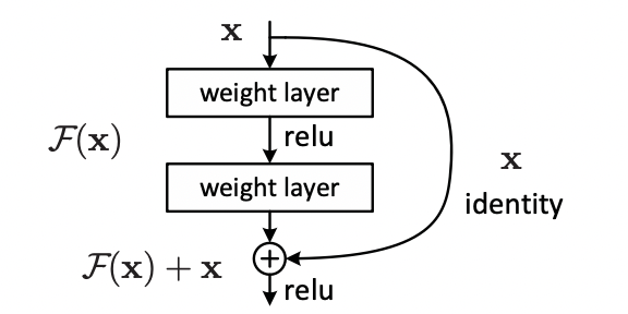
FIGURE 2.24: Building block of residual learning (He et al. 2015).

The function $F \left( x,\left\{ W_i\right\} \right)$ represents the residual mapping that is to be learned. For the example with two layers from Figure 2.24, $F = W_2\sigma\left( W_1x\right)$ in which $\sigma$ denotes the ReLU activation function. Biases are left out to simplify the notation. The operation $F + x$ is conducted with a shortcut connection and element-wise addition. Afterward, a second non-linear (i.e., $\sigma \left( y \right)$ transformation is applied.

The shortcut connections in Equation (2.1) neither adds an extra parameter nor increases computation complexity and enables a comparisons between plain and residual networks that concurrently have the same number of parameters, depth, width, and computational cost (except for the negligible element-wise addition). The dimensions of $x$ and $F$ in Equation (2.1) must be equal. Alternatively, to match the dimensions, linear projection $W_s$ by the shortcut connections can be applied:

\[\begin{equation} \tag{2.2} y = F \left( x,\left\{ W_i\right\} \right)+ W_sx. \end{equation}\]

The square matrix $W_s$ can be used in Equation (2.2). However, experiments showed that identity mapping is enough to solve the degradation problem. Therefore, $W_s$ only aims to match the dimensions. Although more levels are possible, it was experimented with function $F$ having two or three layers without stating the exact form of it. Assuming $F$ only has one layer (Equation (2.1)) it is comparable to a linear layer: $y = W_1 x + x$. The theoretical notations are about fully-connected layers, but convolutional layers were used. The function $F \left( x,\left\{ W_i\right\} \right)$ can be applied to represent multiple convolutional layers. Two feature maps are added element-wise, channel by channel.

2.2.4.2 Network Architectures

Various plain/residual networks were tested to construct an efficient residual network. They trained the network on benchmarked datasets, e.g. the ImageNet dataset, that are used for a comparison of network architectures. Figure (2.2) shows that every residual network needs a plain baseline network inspired by the VGG (Simonyan and Zisserman 2014) network on which identity mapping by shortcuts is applied.

Plain Network: The philosophy of VGG nets 41 mainly inspires the plain baselines. Two rules convolution layers, which usually have $3\times 3$ filters, follow are:

feature maps with the same output size have the same number of layers;
reducing the size of a feature map by half doubles the number of filters per layer to maintain time complexity per layer.

Convolutional layers with a stride of 2 perform downsampling directly. A global average pooling layer and a 1000-way fully-connected layer with softmax are at the end of the network. The number of weighted layers sums up to 34 (Figure 2.25, middle). Compared to VGG nets, this model has fewer filters and lower complexity (Figure 2.25, left).

Residual Network: Based on the above plain network, additional shortcut connections (Figure 2.25, right) turn the network into its associate residual variant. The identity shortcuts (Equation (2.1)) can be directly used in the case of the exact dimensions of the input and output (solid line shortcuts in Figure 2.25). For the different dimensions (dotted line shortcuts in Figure 2.25), two options are considered:

The shortcut still performs identity mapping, but with extra zero entries padded to cope with the increasing dimensions, without adding new parameters;
The projection shortcut in Equation (2.2) matches dimensions (due to $1\times 1$ convolutions).

In both cases, shortcuts will be done with a stride of two when they go across feature maps of two sizes.

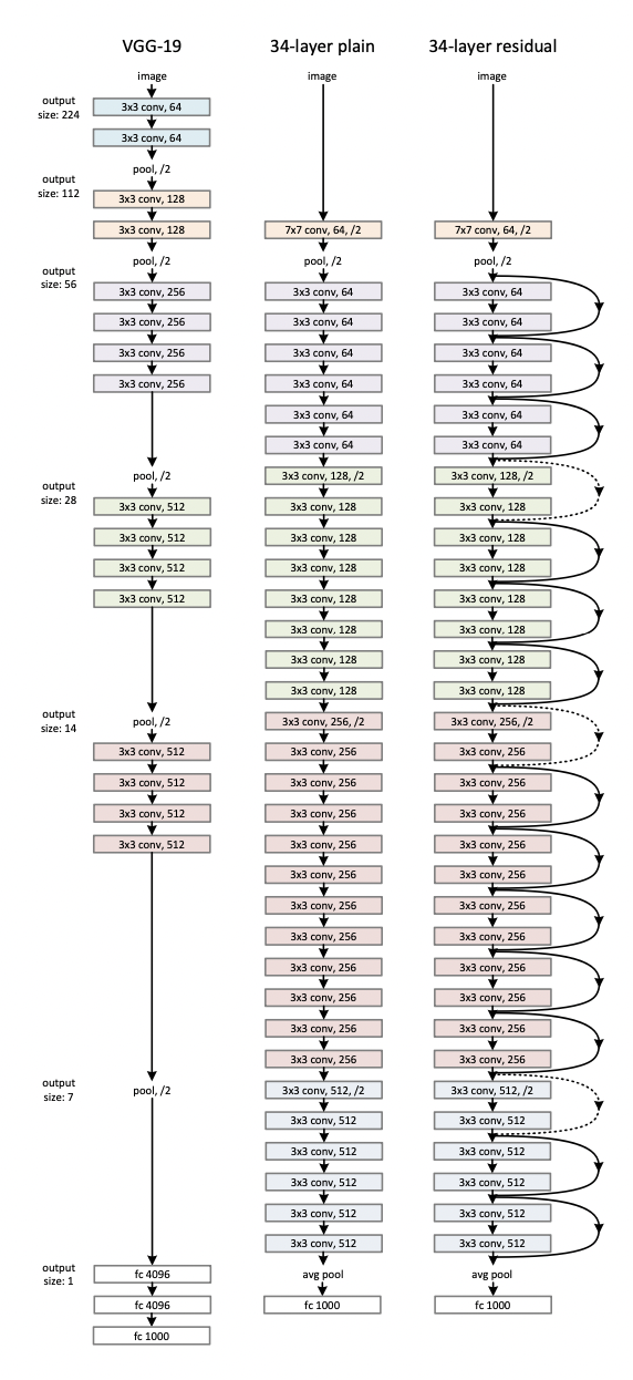
FIGURE 2.25: Architecture of ResNet (He et al. 2015).

2.2.5 EfficientNet

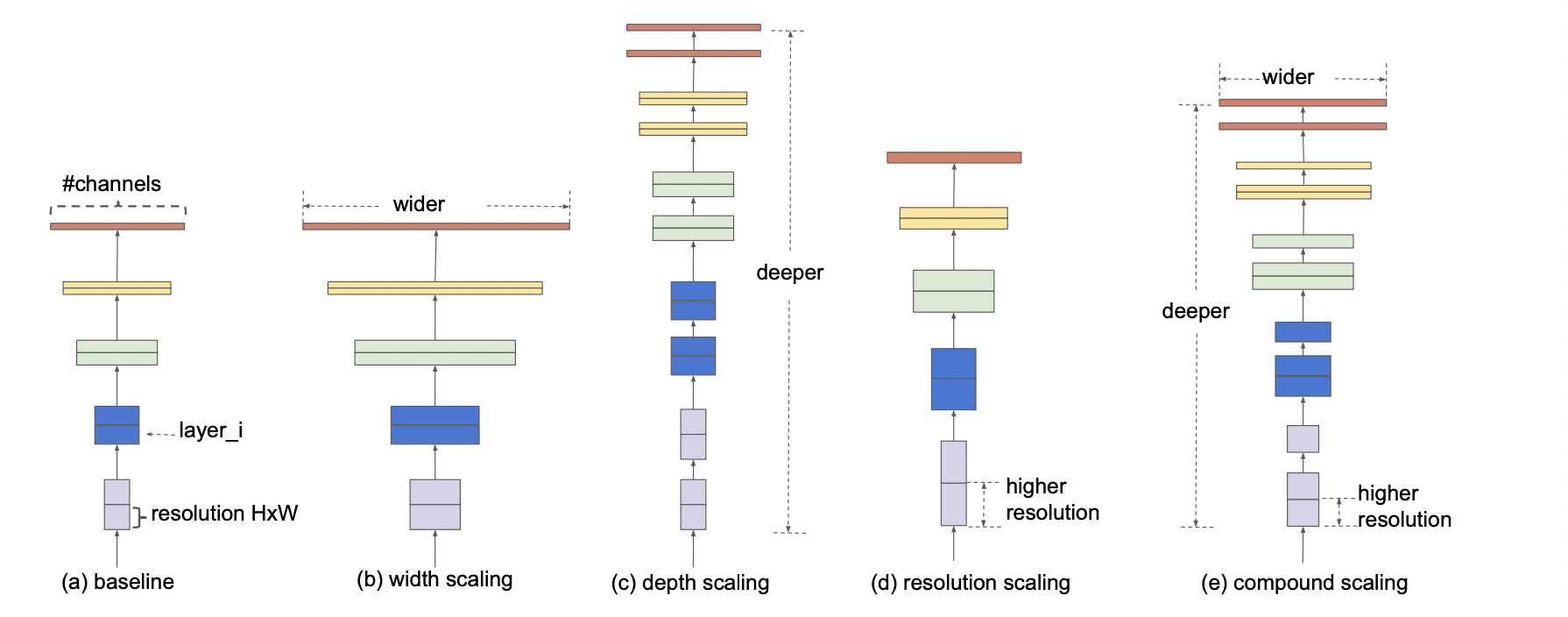
Until (???) introduced EfficientNet, it was popular to scale only one of the three dimensions – depth, width, or image size. The empirical study shows that it is critical to balance all network dimensions, which can be achieved by simply scaling each with a constant ratio. Based on this observation, a simple yet effective compound scaling method was proposed, which uniformly scales network width, depth, and resolution with a set of fixed scaling coefficients. For example, if $2N$ times more computational resources are available, increasing the network depth by $\alpha N$, width by $\beta N$, and image size by $\gamma N$ would be possible. Here $\alpha,\beta,\gamma$ are constant coefficients determined by a small grid search on the original miniature model. Figure 2.26 illustrates the difference between this scaling method and conventional methods. A compound scaling method makes sense if an input image is bigger because a larger receptive field requires more layers and more significant channel features to capture fine-grained patterns. Theoretically and empirically, there has been a special relationship between network width and depth (Raghu et al. 2016). Existing MobileNets (Howard et al. 2017) and ResNets are used to demonstrated new scaling methods.

FIGURE 2.26: Model scaling (M. Tan and Le 2019 b).

2.2.5.1 Compound Model Scaling

2.2.5.1.1 Problem Formulation

A function $Y_i = \mathcal{F}_i \left( X_i \right)$ with the operator $\mathcal{F}_i$, output tensor $Y_i$, input tensor $X_i$ of shape $\left( H_i, W_i, C_i \right)$, spatial dimensions $H_i$, $W_i$, and channel dimension $C_i$ is called a ConvNet Layer $i$. A ConvNet N appears as a list of composing layers: \[ \mathcal{N}=\mathcal{F_k}\odot \cdots \mathcal{F_2}\odot\mathcal{F_1}\left( X_1 \right)=\bigodot{j=1\cdots k}\mathcal{F_j}\left( X_1 \right) \]

Effectively, these layers are often partitioned into multiple stages and all layers in each stage share the same architecture. For example, ResNet has five stages with all layers in every stage being the same convolutional type except for the first layer that performs down-sampling. Therefore, a ConvNet can be defined as:

\[ \mathcal{N}=\bigodot_{i=1\cdots s}\mathcal{F_i}^{L_i}\left( X_{\left( H_i, W_i, C_i \right)} \right) \]

where $\mathcal{F_i}^{L_i}$ denotes layer $\mathcal{F_i}$ which is repeated $L_i$ times in stage $i$, and $\left( H_i, W_i, C_i \right)$ is the shape of input tensor $X$ of layer $i$.

In comparison to the regular ConvNet focusing on the best layer architecture search $\mathcal{F_i}$, model scaling centers on the expansion of the network length $\left( L_i\right)$, width $\left( C_i \right)$, and/or resolution $\left( H_i, W_i\right)$ without changing $\mathcal{F_i}$ that was predefined in the baseline network. Although model scaling simplifies the design problem of the new resource constraints through fixing $\mathcal{F_i}$, a different large design space $\left( L_i, H_i, W_i, C_i \right)$ for each layer remains to be explored. To further reduce the design space, all layers are restricted to be scaled uniformly with a constant ratio. In this case, the goal is to maximize the model’s accuracy for any given resource constraint, which is presented as an optimization problem:

\[\begin{align*} \max_{d,w,r} &\text{Accuracy} \left( \mathcal{N}\left( d,w,r \right) \right) \\ s.t.\mathcal{N}\left( d,w,r \right) &=\bigodot_{I=1...s}\hat{\mathcal{F}}{i}^{d\cdot \hat{L{i}}}\left( X_{\left\langle r\cdot \hat{H_i},r\cdot \hat{W_i},w\cdot \hat{C_i}\right\rangle} \right) \\ Memory\left( \mathcal{N} \right) &\leq\ targetMemory \\ FLOPS\left( \mathcal{N} \right) &\leq\ targetFlops \end{align*}\] where $w,d,r$ are coefficients for scaling network width, depth, and resolution; $\left(\widehat{\mathcal{F}}_i, \widehat{L}_i, \widehat{H}_i, \widehat{W}_i, \widehat{C}_i \right)$ are predefined parameters of the baseline network.

2.2.5.1.2 Scaling Dimensions

The main difficulty of this optimization problem is that the optimal $d, w, r$ depend on each other and the values are changing under different resource constraints. Due to this difficulty, conventional methods mostly scale ConvNets in one of these dimensions:

Depth ($d$): One of the most significant networks previously described is the ResNet. As it was described, the problem of ResNets is that accuracy gain of a very deep network diminishes. For example, ResNet-1000 has similar accuracy to ResNet-101 even though it contains many more layers.

Width ($w$): Scaling network width is commonly used for small-sized models. However, wide but shallow networks tend to have difficulty grasping higher-level features.

Resolution ($r$): Starting from $224\times 224$ in early ConvNets, modern ConvNets tend to use $299\times 299$ or $331\times 331$ for better accuracy. GPipe (Huang et al. 2018) recently achieved state-of-the-art ImageNet accuracy with $480\times 480$ resolution. Higher resolutions, such as $600\times 600$, are also widely used in ConvNets for object detection.

The above analyses lead to the first observation:

Observation 1: Scaling up any network width, depth, or resolution dimension improves accuracy. Without the upscaling, the gain diminishes for bigger models.

2.2.5.1.3 Compound Scaling

Firstly, it was observed that different scaling dimensions are not independent because higher resolution images also require to increase the network depth. The larger receptive fields can help capture similar features that include more pixels in bigger images. Similarly, network width should be increased when the resolution is higher to capture more fine-grained patterns. The intuition suggests that different scaling dimensions should be coordinated and balanced rather than conventional scaling in single dimensions. To confirm this thought, results of networks with width $w$ without changing depth ($d$=1.0) and resolution ($r$=1.0) were compared with deeper ($d$=2.0) and higher resolution ($r$=2.0) networks. This showed that width scaling achieves much better accuracy under the same FLOPS. These results lead to the second observation:

Observation 2: To achieve better accuracy and efficiency, balancing the network width, depth, and resolution dimensions during ConvNet scaling is critical. Earlier researches have tried to arbitrarily balance network width and depth, but they all require tedious manual tuning.

A new compound scaling method, which uses a compound coefficient $\varphi$ to uniformly scale network width, depth, and resolution in a principled way was proposed:

\[\begin{align} \begin{split} \text{depth:} &\mathcal{d}=\alpha^{\varphi} \\ \text{width:} &\mathcal{w}=\beta^{\varphi}\\ \text{resolution:} &\mathcal{r}=\gamma^{\varphi}\\ &s.t. \alpha\cdot \beta^{2}\cdot \gamma^{2}\approx 2\\ &\alpha \ge 1, \beta \ge 1, \gamma \ge 1 \end{split} \tag{2.3} \end{align}\]

where $\alpha, \beta, \gamma$ are constants that can be determined by a small grid search, $\varphi$ is a user-specified coefficient that controls how many more resources are available for model scaling, while $\alpha, \beta, \gamma$ specify how to assign these extra resources to the network width, depth, and resolution, respectively. Notably, the FLOPS of a regular convolution operation is proportional to $d, w^{2}, r^{2}$, i.e., doubling network depth will double the FLOPS, but doubling network width or resolution will increase the FLOPS by four times. Scaling a ConvNet following Equation (2.3) will approximately increase the total number of FLOPS by $\left( \alpha\cdot \beta^{2}\cdot \gamma^{2} \right)^{\varphi}$. In this chapter, $\alpha\cdot \beta^{2}\cdot \gamma^{2}\approx 2$ is constrained such that for any new $\varphi$ the total number of FLOPS will approximately increase by $2\varphi$.

2.2.5.2 EfficientNet Architecture

A good baseline network is essential because model scaling does not affect its layer operators $F*[i]$. Therefore this method is also estimated on ConvNets. A new mobile-sized baseline called EfficientNet was developed to show the effectiveness of the new scaling method. Metrics that were used to estimate the efficacy are accuracy and FLOPS. The baseline efficient network that was created is named EfficientNet-B0. Afterwards, this compound scaling method is applied in two steps:

STEP 1: By fixing $\varphi = 1$ and, assuming twice more resources available, a small grid search of $, , $ based on Equation (2.3) showed that the best values for EfficientNet-B0 are $\alpha = 1.2, \beta = 1.1, \gamma=1.15$ under the constraint of $\alpha·\beta^2·\gamma^2 ≈2$.
STEP 2: Afterwards, fix $\alpha,\beta,\gamma$ as constants and scale up the baseline network with different $\varphi$ using Equation (2.3) to construct EfficientNet-B1 to B7.

Name	Number of parameters
EfficientNet-B0	5.3M parameters
EfficientNet-B1	7.8M parameters
EfficientNet-B2	9.2M parameters
EfficientNet-B3	12M parameters
EfficientNet-B4	19M parameters
EfficientNet-B5	30M parameters
EfficientNet-B6	43M parameters
EfficientNet-B7	66M parameters

Indeed, even better performance is achievable by searching for $\alpha,\beta,\gamma$ directly around a large model, but the search cost becomes prohibitively more expensive on larger models. This method searches once on a small baseline network, then scales the coefficient for all other models.

2.2.5.3 Results and comparison of the networks

To demonstrate the performance of both networks, ResNet and EfficientNets were trained and evaluated on the ImageNet 2012 classification dataset consisting out of 1000 classes. Since deeper scaling should provide better results in the case of ResNet, it was trained with increased depth each time. First meaningful results were obtained in ResNet-34, which performed 3.5 % better than plain-34 baseline when top-1 accuracy is compared. They also compared three versions of ResNet: (A) zero-padding shortcuts (increasing dimensions, all shortcuts are parameter-free) (B) projection shortcuts (increasing dimensions, other shortcuts are identity), and (C) all shortcuts are projections. Each version improved both, the top-1 and top-5 accuracy. Afterward, the depth of the network was increased and ResNet-50, ResNet-101, and ResNet-152 were created. Each increase in depth leads to higher accuracy. In deeper models, the trade-off between accuracy increase and deeper model is not worth describing. All results are shown in the following table:

Model	top-1 acc.	top-5 acc.
VGG-16	71.93	90.67
GoogLeNet	-	90.85
plain-34	71.46	89.98
ResNet-34 A	74.97	92.24
ResNet-34 B	75.48	92.54
ResNet-34 C	75.81	92.6
ResNet-50	77.15	93.29
ResNet-101	78.25	93.95
ResNet-152	78.57	94.29

In the case of EfficientNets, the results achieved by the previous state-of-the-art networks on the same ImageNet dataset were aimed to improve. Among all state-of-the-art networks, EfficientNets were compared with ResNets-50 and ResNet-152. They compared the results of networks deviated by changing scaling parameters EfficientNet-B0 to EfficientNet-B7. The results of each network were better than the previous one. Also, they have shown that EfficientNet-B0 outperforms ResNet-50 and that EfficientNet-B1 outperforms ResNet-152. This means that scaling through all three dimensions can provide better results than scaling through just one dimension. The drawback of this approach is the computational power which makes it less popular than the previous methods. Again, all results are shown in the following table:

Model	top-1 acc.	top-5 acc.
EfficientNet-B0 / ResNet-50	77.1 / 76	93.3 / 93
EfficientNet-B1 / ResNet-152	79.1 / 77.8	94.4 / 93.8
EfficientNet-B2	80.1	94.9
EfficientNet-B3 / ResNeXt-101	81.6 / 80.9	95.7 / 95.6
EfficientNet-B4	82.9	96.4
EfficientNet-B5	83.6	96.7
EfficientNet-B6	84	96.8
EfficientNet-B7 / GPipe	84.3 / 84.3	97 / 97

2.2.6 Contrastive learning

In recent years the problem of classification of unlabeled dataset is becoming more widespread. More unlabeled datasets requiring human labeling are created in fields like medicine, the automotive industry, military, etc. Since the process is expensive and time-consuming, researchers assumed it could be automated with contrastive learning frameworks. One of the first and most known contrastive learning frameworks is SimCLR (T. Chen, Kornblith, Norouzi, and Hinton 2020 a). The advantage of this framework is its simplicity, yet it achieves high accuracy on classification tasks. The main idea is to have two copies of the image, which are then used to train two networks and that are compared. The problem with this framework is that it doubles the size of the dataset and reaches among all images, which can be computationally infeasible for large datasets. Bootstrap Your Own Latent (Grill, Strub, Altché, et al. 2020) was introduced to avoid making double-sized datasets. The idea was to bootstrap image representations to avoid unnecessary image comparisons. These two frameworks will be described in this chapter.

Further improvements in the choice of creating two views of images and comparison techniques were presented in different frameworks such as Nearest-Neighbor Contrastive Learning (NNCLR) (Dwibedi et al. 2021), Open World Object Detection (ORE) (Joseph et al. 2021), Swapping Assignments between multiple Views (SwAV) {Caron et al. (2020)}, and many more. This field is a constant research topic and new improved frameworks are proposed on a constant basis to help researchers solve different tasks that requires labeled datasets.

2.2.6.1 A Simple Framework for Contrastive Learning of Visual Representations

T. Chen, Kornblith, Norouzi, and Hinton (2020 a) intended to analyze and describe a better approach to learning visual representations without human supervision. They have introduced a simple framework for contrastive learning of visual representations called SimCLR. As they claim, SimCLR outperforms previous work, is more straightforward, and does not require a memory bank.

Intending to understand what qualifies good contrastive representation learning, the significant components of the framework were studied and resulted in:

A contrastive prediction task requires combining multiple data augmentation operations, which results in effective representations. Unsupervised contrastive learning benefits from more significant data augmentation.
The quality of the learned representations can be substantially improved by introducing a learn-able non-linear transformation between the representation and the contrastive loss.
Representation learning with contrastive cross-entropy loss can be improved by normalizing embeddings and adjusting the temperature parameter appropriately.
Unlike its supervised counterpart, contrastive learning benefits from larger batch sizes and extended training periods. Contrastive learning also benefits from deeper and broader networks, just as supervised learning does.

2.2.6.2 The Contrastive Learning Framework

Like for SimCLR, a contrastive loss is used to learn a representation by maximizing the agreement between various augmented views of the same data example. This framework contains four significant components, which are shown in Figure ??:

A stochastic data augmentation module
A neural network base encoder
A small neural network projection head
A contrastive loss function

FIGURE 2.27: A simple framework for contrastive learning of visual representations (T. Chen, Kornblith, Norouzi, and Hinton 2020 a).

2.2.6.2.1 Stochastic data augmentation module

First, the minibatch of $N$ examples is sampled randomly, and the contrastive prediction task is defined on pairs of augmented examples, resulting in $2N$ data points. A memory bank was not used to train the model, instead, the training batch size varies from 256 to 8192. Any given data example randomly returns two correlated views of the same example, denoted $\tilde{x}_{i}$ and $\tilde{x}_{j}$, which is known as a positive pair. Negative pairs are all other $2(N-1)$ pairs. In one view, some data augmentation techniques are applied. Data augmentation is widely embraced in supervised and unsupervised representation learning. Unfortunately, it has not been used to define the contrastive prediction task, which is mainly determined by changing the architecture. It was shown that choosing different data augmentation techniques can reduce the complexity of previous contrastive learning frameworks. There are many data augmentation operations, the focus was on the most common ones, which are:

Spatial geometric transformation: cropping and resizing (with horizontal flipping), rotation and cutout,
Appearance transformation: color distortion (including color dropping), brightness, contrast, saturation, Gaussian blur, and Sobel filtering.

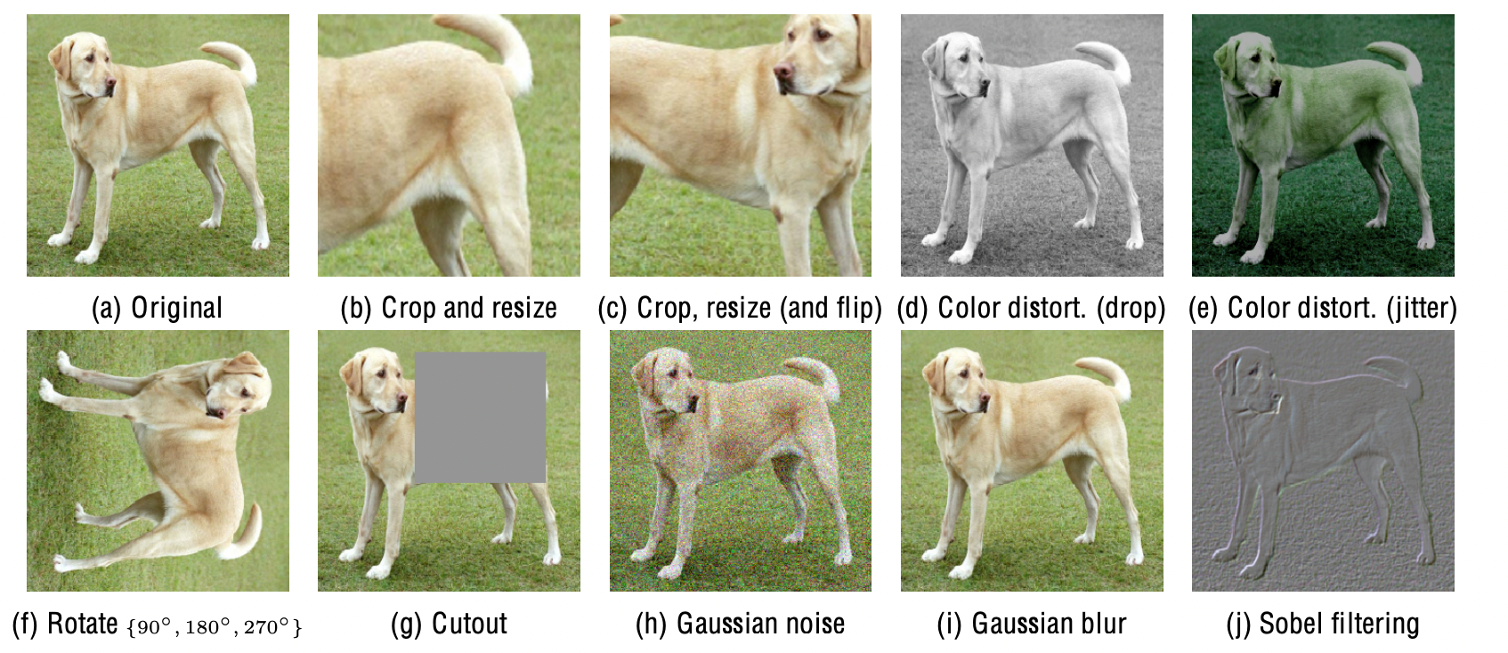
FIGURE 2.28: Augmentation texhniques (T. Chen, Kornblith, Norouzi, and Hinton 2020 a).

Due to the image sizes in the ImageNet dataset, all images were always randomly cropped and resized to the same resolution. Later on, other targeted data augmentation transformations were applied to one branch, remaining the one as original i.e. $t\left( x_{i}\right)= x_i$. Applying just individual transformation is insufficient for the model to learn good representations. The model’s performance improves after composing augmentations, although the contrastive prediction task becomes more complex. The composition of augmentations that stood out were random cropping and random color distortion.

It was also observed that stronger color augmentation significantly improves the linear evaluation of unsupervised learned models. Stronger color augmentations do not enhance the performance of supervised learning models when trained with the same augmentations. Based on the experiments, unsupervised contrastive learning benefits from stronger color data augmentation than supervised learning.

2.2.6.2.2 Neural network base encoder

Neural network based encoder $f\left( \cdot \right)$ extracts multiple representation vectors from the augmented data examples. This framework does not restrict a choice of the network architecture, although for simplicity, the commonly used ResNet was picked and gives $h_i=f\left( \tilde{x}_{i} \right)=ResNet\left(\tilde{x}_{i}\right)$ where $\textbf{h}_i\in \mathbb{R}^{d}$ is the output after the average pooling layer. Although increasing depth and width improves performance, the ResNet-50 was chosen. Furthermore, when the model size increases, the gap between supervised and unsupervised learning shrinks, suggesting that bigger models benefit more from unsupervised learning.

2.2.6.2.3 Small neural network projection head

A small neural network projection head $g\left( \cdot \right)$ maps the representation to the space where the contrastive loss is applied to. The importance of including a projection head, i.e., $g\left( h \right)$ was evaluated and they considered three different architectures for the head:

identity mapping,
linear projection,
the default non-linear projection with one additional hidden layer and ReLU activation function.

The results showed that a non-linear projection head is better than a linear projection and much better than no projection. It improves the representation quality of the layer that is applied previous to it. They have used a MLP with one hidden layer to obtain $z_i = g\left( \textbf{h}_i \right) = W^{\left( 2\right)}\sigma \left( W^{\left( 1\right)} \textbf{h}_i\right)$ where $\sigma$ is a ReLU non-linearity transformation.

This step is performed because defining the contrastive loss on $z_i$ instead of on $\textbf{h}_i$ would not lead to a loss of information caused by contrastive loss. Especially, $z=g\left( h \right)$ is trained to be invariant to data transformations. As a result, $g$ can remove information useful for a downstream task such as object color or orientation. Using the non-linear transformation $g\left( * \right)$, $h$ can maintain and form more information.

2.2.6.2.4 Contrastive loss function

Given a set $\left\{ \tilde{x}_{ik} \right\}$ including a positive pair of examples $\tilde{x}_{i}$ and $\tilde{x}_{j}$, the contrastive prediction task aims to identify $\tilde{x}_{i}$ in $\left\{ \tilde{x}_{i} \right\}_{k\neq i}$ for a given $\tilde{x}_{i}$. In the case of positive examples, the loss function is defined as \[ \mathcal{l}_{i,j} = −\log\frac{exp\left( \frac{sim(z_i,z_j)}{\tau} \right)}{\sum_{k=1}^{2N}\mathbb{I_{\left[ k\neq i \right]}}exp\left( \frac{sim(z_i,z_k)}{\tau} \right)} \]

where $\mathbb{I_{\left[ k\neq i \right]}}\in\left\{ 0,1 \right\}$ is an indicator function, $\tau$ denotes a temperature parameter and $sim\left(\textbf{u,v} \right)= \frac{\textbf{u}^T\textbf{v}}{\left\| \textbf{u}\right\|\left\| \textbf{v} \right\|}$ is a dot product between $\mathcal{l}_2$ and normalized $\textbf{u},\textbf{v}$.

The final loss is calculated across all positive pairs, both $\left( i,j \right)$ and $\left( j,i \right)$, in a mini-batch. It was named NT-Xent, the normalized temperature-scaled cross-entropy loss.

The NT-Xent loss was compared against other commonly used contrastive loss functions, such as logistic loss and margin loss. Gradient analysis shows that $l_2$ normalization, cosine similarity, and temperature together effectively weight different examples and a suitable temperature can make the model learn from hard negatives. The advantage of NT-Xent is that it weights the negatives by their relative hardness. Without normalization and proper temperature scaling the performance is significantly worse. Also, the contrastive task accuracy is higher, but the resulting representation is worse under linear evaluation.

2.2.6.3 Bootstrap Your Own Latent

The fundamental idea of contrastive learning is to create pairs of images on which the framework would be trained. Creating negative pairs relies on large batch sizes, memory banks, or customized mining strategies which can be challenging in larger datasets. Grill, Strub, Altché, et al. (2020) wanted to create a new approach that would achieve better performance than other contrastive methods without using negative pairs. A solution they have introduced is a method called Bootstrap Your Own Latent (BYOL). The idea was to bootstrap representations of images. As a result, BYOL is more robust to the choice of image augmentations. Furthermore, BYOL has two neural networks, called online and target network, who interact and learn from each other. Using an augmented view of an image, BYOL trains its online network to predict the target network’s representation of another augmented view. This approach achieved state-of-the-art results when trained on the ImageNet dataset under the linear evaluation protocol. Additionally, compared to SimCLR, a strong contrastive baseline, BYOL suffers from much less performance drop when only random crops are used to augment images.

2.2.6.3.1 Description of the method

BYOL aims to learn a representation of $y_\theta$. It uses two neural networks: online and the target network to achieve that. The online network is determined by a set of weights $\theta$ and consists of:

an encoder $f_\theta$,
a projector $g_\theta$,
a predictor $q_\theta$.

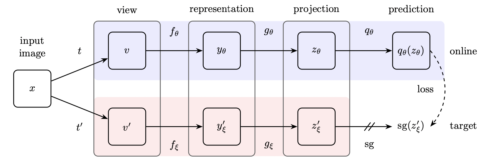
FIGURE 2.29: Bootstrap Your Own Latent (Grill, Strub, Altché, et al. 2020).

The target network has the same architecture as the online network but uses different weights $\xi$. It provides the regression targets to train the online network, and its parameters $\xi$ are an exponential moving average of the online parameters $\theta$. Precisely, given a target decay rate $\tau \in[0,1]$, after each training step, the following update

\[ \xi \leftarrow \tau \xi+(1-\tau) \theta \]

is performed. Firstly, an image is sampled uniformly from $\mathcal{D}$ from which two distributions of image augmentations $\mathcal{T}$ and $\mathcal{T}^{\prime}$ are created. BYOL applies respectively two image augmentations $t \sim \mathcal{T}$ and $t^{\prime} \sim \mathcal{T}^{\prime}$ creating two augmented views $v \triangleq t(x)$ and $v^{\prime} \triangleq t^{\prime}(x)$. First augmented view $v$ is used for the online network and result in the output $y_{\theta} \triangleq f_{\theta}(v)$ and afterwards the projection $z_{\theta} \triangleq g_{\theta}(y)$. Similarly, from the second augmented view $v^{\prime}$ the target network outputs $y_{\xi}^{\prime} \triangleq f_{\xi}(v^{\prime})$ and the target projection $z_{\xi}^{\prime} \triangleq g_{\xi}(y^{\prime})$. Later on output a prediction of $q_{\theta}\left(z_{\theta}\right)$ of $z_{\xi}^{\prime}$ and $\ell_{2}$-normalize both $q_{\theta}\left(z_{\theta}\right)$ and $z_{\xi}^{\prime}$ to

\[ \overline{q_{\theta}}\left(z_{\theta}\right) \triangleq q_{\theta}\left(z_{\theta}\right) /\left\|q_{\theta}\left(z_{\theta}\right)\right\|_{2} \quad \textrm{and} \quad \bar{z}_{\xi}^{\prime} \triangleq z_{\xi}^{\prime} /\left\|z_{\xi}^{\prime}\right\|_{2}. \]

The predictor is only applied to the online pipeline, making the architecture asymmetric between the online and target pipeline. Lastly, the following mean squared error between the normalized predictions and target projections is defined:

\[ \mathcal{L}_{\theta, \xi} \triangleq\left\|\overline{q_{\theta}}\left(z_{\theta}\right)-\bar{z}_{\xi}^{\prime}\right\|_{2}^{2}=2-2 \cdot \frac{\left\langle q_{\theta}\left(z_{\theta}\right), z_{\xi}^{\prime}\right\rangle}{\left\|q_{\theta}\left(z_{\theta}\right)\right\|_{2} \cdot\left\|z_{\xi}^{\prime}\right\|_{2}} \]

The loss is symmetrized $\mathcal{L}_{\theta, \xi}$ by using $v^{\prime}$ for the online network and $v$ for the target network separately to calculate $\widetilde{\mathcal{L}}_{\theta, \xi}$. At each training step, a stochastic optimization step is applied to minimize $\mathcal{L}_{\theta, \xi}^{\mathrm{BYOL}}=\mathcal{L}_{\theta, \xi}+\widetilde{\mathcal{L}}_{\theta, \xi}$ with respect to $\theta$ only but not $\xi$. BYOL’s dynamics are summarized as

\[ \theta \leftarrow \operatorname{optimizer}\left(\theta, \nabla_{\theta} \mathcal{L}_{\theta, \xi}^{\mathrm{BYOL}}, \eta\right). \]

where $\eta$ is a learning rate. At the end of the training, only the encoder $f_{\theta}$ is used.

2.2.6.4 Comparison of contrastive learning frameworks

Of all frameworks, SimCLR is the most popular due to its simplicity. The ResNet-50 in 3 different hidden layer widths (width multipliers of $1\times$, $2\times$, and $4\times$) were used and trained for 1000 epochs each. The accuracy of these frameworks on the ImageNet dataset with few labels improved when the width of ResNet-50 increases. For SimCLR with ResNet-50 top-1 accuracy is 69.3 and top-5 accuracy is 89, while for ResNet-50(4x) top-1 accuracy is 85.8 and top-5 accuracy is 92.6. These results are comparable with supervised methods. The BYOL framework was built to improve the results of SimCLR. It was also stated that the accuracy for the baseline ResNet-50 is 74.3 and 91.6 for top-1 accuracy and top-5 accuracy. When using ResNet-50(4x), an increase in accuracy to 78.6 and 94.2 for top-1 and top-5 is observed, respectively. More information about performance can be found in following table:

Model	Architecture	Param (M)	top-1 acc.	top-5 acc.
SimCLR	ResNet-50	24	69.3	89.0
SimCLR	ResNet-50 (2x)	94	74.2	93.0
SimCLR	ResNet-50 (4x)	375	76.5	93.2
BYOL	ResNet-50	24	74.3	91.6
BYOL	ResNet-50 (x2)	94	77.4	93.6
BYOL	ResNet-50 (x4)	375	78.6	94.2
BYOL	ResNet-200 (x2)	250	79.6	94.8

2.2.7 Transformers in Computer Vision

Since the first appearance of the Transformers architecture in 2017 (???), it has become an irreplaceable part of all-natural language processing (NLP) models. The main advantage of Transformers is that they can be trained on a large text corpus and then fine-tuned on a smaller task-specific dataset. This enabled model training of unspecified size with more than 100B parameters.

However, computer vision still relied on convolutional architectures. With datasets constantly growing and the diversity of the fields computer vision tasks could be applied to, researchers wanted to implement Transformers architecture in the CV field. Some works aim for combining CNN-like architectures with self-attention (J. Wang and Li 2018). Others attempted to replace convolutions entirely, e.g. Ramachandran et al. (2019). Due to specialized attention patterns, the problem was that they have not yet been scaled effectively on modern hardware accelerators. Therefore, in large-scale image recognition, classic ResNet-like architectures are still state-of-the-art.

In 2021 the Google research Brain Team published the paper “An image is worth $16\times 16$ words” where they introduced new Transformers-based architecture for CV called Vision Transformers (ViT) (Dosovitskiy, Beyer, Kolesnikov, Weissenborn, Zhai, Unterthiner, Dehghani, Minderer, Heigold, Gelly, Uszkoreit, et al. 2020 b). Based on the success of Transformer in NLP scaling, they aimed to apply standard Transformer directly to images with little as possible changes to the existing architecture. The image is split into patches and linear embeddings of these patches are provided as inputs to the Transformer. These patches are the same as tokens (e.g. words) in NLP. The model is trained for image classification in a supervised learning fashion.

2.2.7.1 Vision Transformers

Brain Team wanted to create simple but universally scalable architecture to follow the original Transformers architecture.

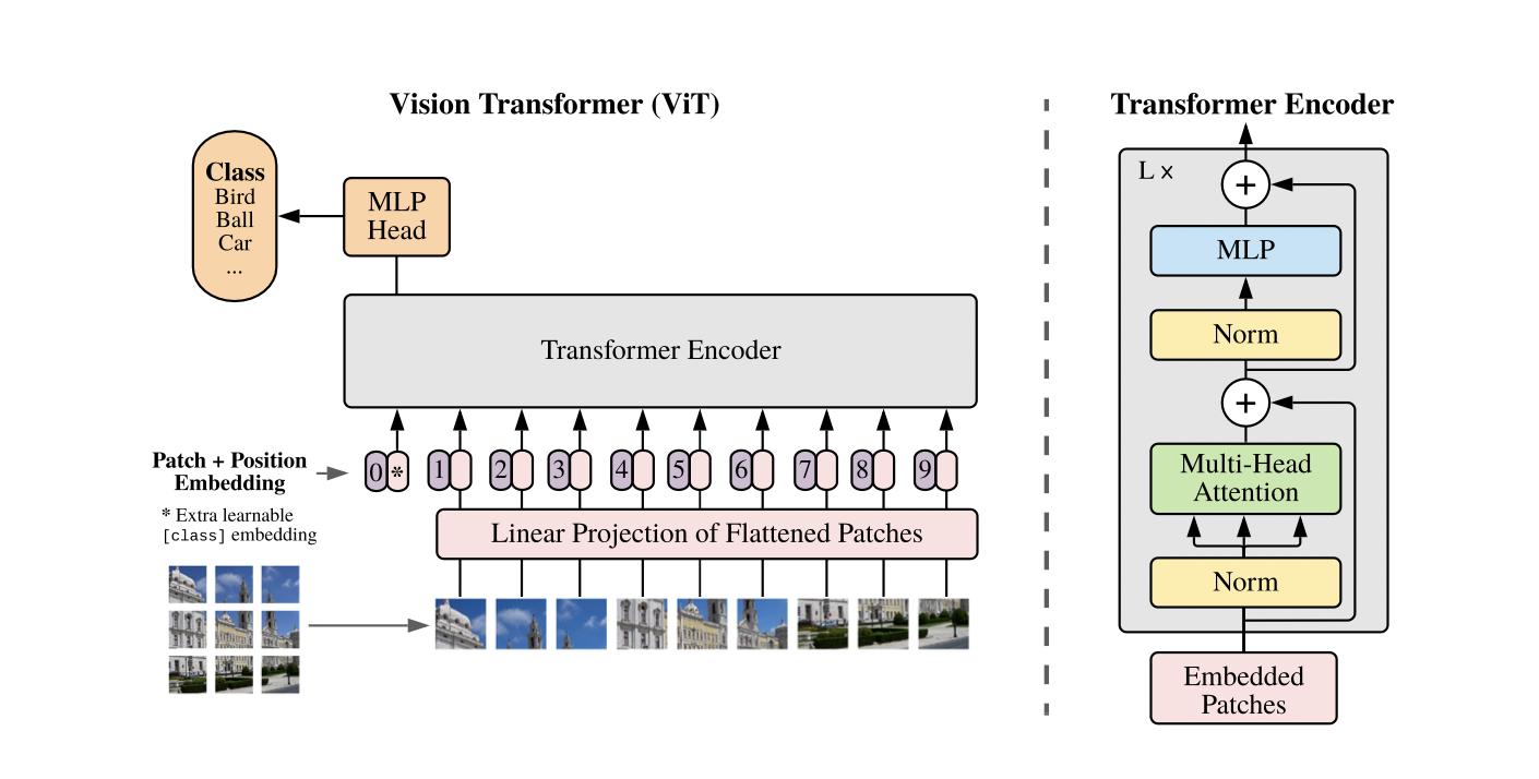
Vision Transformer (Dosovitskiy, Beyer, Kolesnikov, Weissenborn, Zhai, Unterthiner, Dehghani, Minderer, Heigold, Gelly, Uszkoreit, et al. 2020b).

FIGURE 2.30: Vision Transformer (Dosovitskiy, Beyer, Kolesnikov, Weissenborn, Zhai, Unterthiner, Dehghani, Minderer, Heigold, Gelly, Uszkoreit, et al. 2020 b).

2.2.7.1.1 Method

Compared to NLP, with 1-dimensional token embedding input for the Transformer, images are 2-dimensional objects. Firstly, images needed to be represented differently to imitate original architectures as close as possible. For that reason image $x\in \mathbb{R}^{ H \times W \times C}$ is reshaped into a sequence of flattened 2-dimensional patches $x_p\in \mathbb{R}^{ N \times \left( P^2 \cdot C \right)}$, where $\left(H,W\right)$ is the resolution of the original image, $C$ is the number of channels, $\left(P,P\right)$ is the resolution of each image patch, and $N =HW/P^2$ is the resulting number of patches, also the Transformer’s effective input sequence length. The Transformer input through all layers is a fixed vector of size $D$. The first step is to flatten the patches, usually $16\times 16$ and map them to $D$ dimensions with a trainable linear projection to create patch embeddings.

\[ \mathbf{z}_{0} =\left[\mathbf{x}_{\text {class }} ; \mathbf{x}_{p}^{1} \mathbf{E} ; \mathbf{x}_{p}^{2} \mathbf{E} ; \cdots ; \mathbf{x}_{p}^{N} \mathbf{E}\right]+\mathbf{E}_{p o s}, \mathbf{E} \in \mathbb{R}^{\left(P^{2} \cdot C\right) \times D}, \mathbf{E}_{p o s} \in \mathbb{R}^{(N+1) \times D} \]

To this sequence of “patch embeddings”, a prefix learnable [class] token, like in BERT, is usually added. This token $\mathbf{z}_{0}^{0} = \mathbf{x}_{class}$ tells the model to classify the image and increases the dimension of vector $z$. Also, the state of this token at the output of the Transformer encoder $\left(\mathbf{z}_{L}^{0}\right)$, on which the layernorm is applied, serves as the image representation $y$.

\[ \mathbf{y} =\operatorname{LN}\left(\mathbf{z}_{L}^{0}\right) \]

Furthermore, it is the only one to which the classification head is attached to during pre-training and fine-tuning. The classification head during pre-training is compiled of MLP with one hidden layer and a single linear layer at a fine-tuning time. Position embedding, a standard learnable 1-dimensional position embedding, are attached to the patch embeddings, serving as input to the encoder. The standard Transformer encoder consists of alternating layers of multiheaded self-attention and MLP blocks. After each block, a residual connection is applied.

\[ \mathbf{z}_{\ell}^{\prime} =\operatorname{MSA}\left(\operatorname{LN}\left(\mathbf{z}_{\ell-1}\right)\right)+\mathbf{z}_{\ell-1}, \ell=1 \ldots L \]

\[ \mathbf{z}_{\ell} =\operatorname{MLP}\left(\mathrm{LN}\left(\mathbf{z}_{\ell}^{\prime}\right)\right)+\mathbf{z}_{\ell}^{\prime}, \ell=1 \ldots L \]

Vision Transformer has a significantly lower inductive bias than CNNs in image-specific information. VIT only has local and translational equivariant MLP layers, while the self-attention layers are global. A 2-dimensional neighborhood structure is used sparingly: the image is cut into patches at the beginning and the position embeddings are resized as needed at the fine-tuning time. Alternatively, the input sequence can consist of a CNN’s feature map on which the patch embedding projection is applied. Vision Transformers are pre-trained on large datasets and fine-tuned to (smaller) downstream tasks. For fine-tuning, a projection head is removed and a zero-initialized $D \times K$ feedforward layer is attached with $K$ being the number of downstream classes. It is also beneficial to use higher resolution then in pre-training. Also ViT can handle arbitrary sequence lengths but the pre-trained position embeddings can become sufficient. It is necessary to point out that resolution adjustment and patch extraction are the only points at which an inductive bias about the 2-dimensional structure of the images is manually injected into the Vision Transformers

2.2.7.1.2 Experiments

Similarly to BERT models, multiple versions of the model at various scales were created. They have created Base = “B”, Large = “L”, Huge = “H” versions of ViT, with 12, 24 and 32 layers and 86M, 307M and 632M parameters respectively.

To explore the model scalability, the previous mentioned dataset ImageNet was used. In addition, ViT was compared against a slightly modified ResNet called “ResNet(BiT)”. The batch Normalization layer was replaced with Group Normalization and used standardized convolutions. Another network that it was compared to was Noisy Student (Xie et al. 2019), a large EfficientNet. Experiments showed that ViT Hughe with $14\times 14$ input patch size outperformed both CNN-based networks with an accuracy of 88.5%, whereas ResNet BiT had 87.54% and Noisy Student 88.4%. It is worth mentioning that ViT Large with $16\times 16$ input patch size had 87.76% accuracy on the same dataset. Another thing worth pointing out is that ViT outperforms CNN-based architectures on all larger datasets yet performs slightly worse than CNN networks on a smaller dataset.

2.2.8 Conclusion

In this chapter, the authors presented some of the current state-of-the-art approaches in Computer Vision. Nowadays, when technology is advancing each day, creating networks that would imitate human brain is more challenging. Still, the networks presented in this chapter are highly accurate and creating network which can out-perform them is challenging. Furthermore, it is noticeable that the application of CV is dictating the development of networks and frameworks which help humans with their everyday tasks.

2.3 Resources and Benchmarks for NLP, CV and multimodal tasks

Author: Christopher Marquardt

Supervisor: Christian Heumann

When we see athletes perform in their sports we only see the results of their hard work prior or till to the event. Most of the time they casually talk about their off-season, but everybody knows the results are made in the off-season.

Same goes for the models we will see in the later chapters. We are just interested in the results, but why and how does the model come to these results? It has to learn to some key fundamentals of the modality to achieve these results. But how do they get them to perform in such a way or even better? It’s possible to build better architectures and/or use more and new data to achieve this. New data by hand is easy to get but this new data results in a new problem. New data has to be carefully labeled by humans, which can be very expensive by the amount of data. Models which learn from labeled data use the supervised learning strategy. This learning strategy is a bottleneck for future progress, because of the given reason.

But the need for labeling the data isn’t the only problem. Let’s visit the athlete analogy again. Imagine a professional football player has to participate in a professional ski race. He will not be able to compete with the others, because they are trained only to do ski races. Here see the other problem. Models which use supervised learning have shown to perform very well on the task they are trained to do. This means models which learn on carefully labeled data only perform very well on this specific task, but poor on others. Also it’s not possible to label everything in the world.

So the goal is to generate more generalist models which can perform well on different tasks without the need of huge labeled data. Humans are able to perform well on different tasks in a short amount of time. Humans, for example, only need a small amount of hours to learn how to drive a car, even without supervision. On the other hand fully automated driving AI need thousand of hours of data to drive a car. Why do humans learn so fast compared to machines? Humans don’t rely on labeled data, because most of the time humans learn by observation. By this humans generate a basic knowledge of how the world works, which also called common sense. This enables us to learn so much faster compared to machines. Meta AI (Yann and Ishan 2021) believes that self-supervised learning is one of the most promising ways to generate background knowledge and some sort of common sense in AI systems. By self-supervised learning one means a supervised learning algorithm, but it doesn’t need an external supervisor. Self-supervised pre-training differs between the modalities, which means there is not an approach which works in all modalities. The following chapter will inspect on the one hand pre-training resources and the use of them and on the other hand also the benchmarks which are used for Natural Language Processing (NLP), Computer Vision (CV) and ,the combination of both, vision language pre-trained models (VL-PTM).

2.3.1 Datasets

After pointing out that pre-training is very important, one might ask how do the datasets look and how do the different modalities pre-train? At first we will inspect the former one and focus afterwards on the use of the resources. As one might expect NLP models pre-train on text, CV models pre-train on images and VL-PTM pre-train on text image pairs, which can somehow be seen as a combination of NLP and CV. But CV models mostly used labeled data like a picture of a dog with the corresponding single label “dog”. MML datasets can contain several sentences of text which correspond to the given image.

Even if the datasets might be completely different, the procedure to get the data is mostly the same for all of them, because the data is crafted from the internet. This can lead to a problem, since by using this method the resulting dataset might be noisy. One approach for the VL-PTM, for example, is to use CommonCrawl and extract the image plus the alt of an image. The alt is an alternate text for an image, if the image cannot be displayed or for visual impaired people. This seems like a reasonable approach, but the alt is often not very informative about what’s in the image.

Another difference between the modalities is the cardinality of the pre-training data. It’s easy to realize that text is by far easiest to crawl from the internet. This results in huge high-quality massive text data. Some magnitudes smaller are the datasets for CV. Since VL-PTM are pretty new compared to the other modalities it still relatively small, but growing fast. A small downer is that some of the datasets are not public available. The big companies like to keep their models and used datasets private, which hinders the reproducibility, but there are also real open AI competitors like LAION and Eleuther in the field. The next chapter will provide some of the most used pre-training datasets.

2.3.1.1 Natural Language Processing Datasets

2.3.1.1.1 Common Crawl

As already mentioned, extracting text from the internet is rather easy. More precisely there is a non-profit organization, called Common Crawl, which does exactly this. They provide copies of the internet to researchers, companies and individuals at no cost for the purpose of research and analysis. The Common Crawl corpus contains petabytes of data collected since 2008. Every month, Common Crawl releases a snapshot of the web obtained by randomly exploring and sampling URLs. It contains raw web page data, extracted metadata and text extractions. The advantages of Common Crawl come along with their disadvantages. The text is from diverse domains but with varying quality of data. To handle the raw nature of the datasets one often has to use a well-designed extraction and filter to use the datasets appropriately (Gao et al. 2020). GPT-3 ,for example, uses a filtered version of Common Crawl, which consists of 410 billion tokens (Brown et al. 2020). So data for NLP is freely available but one needs to use well-designed extraction and filtering to really use the dataset.

2.3.1.1.2 The Pile

Recent work (Rosset 2020) showed that diversity in training datasets improves general cross-domain knowledge and downstream generalization capability for language models. The Pile (Gao et al. 2020) was introduced to address exactly these results. The Pile contains $22$ sub-datasets, including established NLP datasets, but also several newly introduced ones. The size of the $22$ sub-datasets, which can be categorized roughly into five categories, pile up to around $825$ GB of data. The following treemap shows the distribution of the dataset.

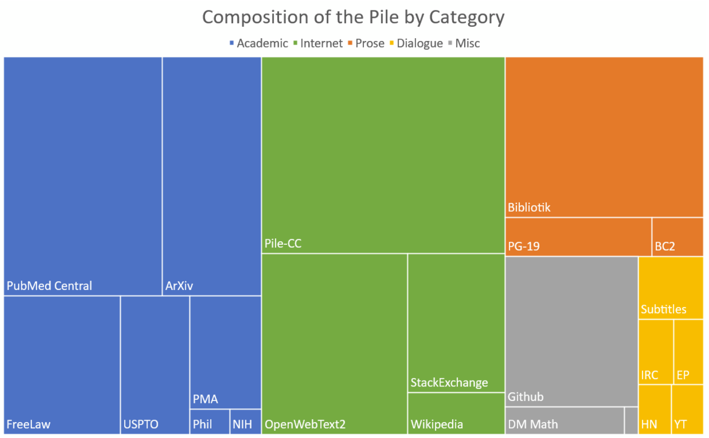
While only 13% of the world’s population speaks English, the vast majority of NLP research is done on English. Gao et al. (2020) followed this trend, but did not explicitly filtered out other languages when collecting our the data. This leads to the fact that roughly 95% of the Pile is English. Also EuroParl (Koehn 2005), a multilingual parallel corpus introduced for machine translation, is included in the Pile. To train GPT-2 Open AI collected data from WebText. WebText is an internet dataset created by scraping URLs extracted from Reddit submissions with a minimum score for quality, but sadly it was never released to the public. Independent researchers reproduced the pipeline and released the resulting dataset, called OpenWebTextCorpus (Gokaslan and Cohen 2019) (OWT). Eleuther created an enhanced version of the original OWT Corpus called OpenWebText2. It covers all Reddit submissions from 2005 up until April 2020. It covers content from multiple languages, document metadata, multiple dataset versions, and open source replication code.

They also explicitly included a dataset of mathematical problems (DeepMind Mathematics) to improve the mathematical ability of language models trained on the Pile. An ArXiv dataset was in included in the hopes that it will be a source of high quality text and math knowledge, and benefit potential downstream applications to research in these areas and also because arXiv papers are written in LaTeX. Training a language model to be able to generate papers written in LaTeX could be a huge benefit to the research community.

Since CC needs further steps, due to the raw nature of CC, to really use is. Pile-CC is Common Crawl-based dataset, which can be used directly. It yields higher quality output than directly using the WET files. These were only some of the 22 included datasets. A more detailed description of the sub-dataset and the reasons why these were included can be found in the corresponding paper (Gao et al. 2020).

2.3.1.1.3 Multilingual Datasets

Another pre-cleaned version of CC is CC-100 (Wenzek et al. 2019). They present a pipeline to create curated monolingual corpora in more than 100 languages. A filter, which covers the data based on their distance to Wikipedia, is used and this improves the quality of the resulting dataset. However, its English portion is much smaller than the Pile. But a multilingual dataset might help a low-resource language acquire extra knowledge from other languages. Perhaps the most multilingual corpus publicly available, containing 30k sentences in over 900 languages, is the Bible corpus (Mayer and Cysouw 2014). Till now all datasets were freely available and almost directly usable. The next one is not public available for some reasons.

To provide mT5 (Xue et al. 2020), which is multilingual pre-trained text-to-text transformer, a suitable pre-training dataset, Google Research designed a dataset including more than 100 languages. The dataset is called mC4 (Xue et al. 2020). Since some languages are relatively scarce on the internet, they used all of the 71 monthly web scrapes released so far by Common Crawl. It contains 6.6 billion pages and 6.3 trillion tokens. A smaller version of the mC4 is also used by Google Research. The smaller dataset C4 (Colossal Clean Common Crawl) was explicitly designed to be English only. The C4 dataset is a collection of about $750$GB of English-language text sourced from the public Common Crawl web.

Most of the datasets used in NLP are derived entirely from Common Crawl and Rosset (2020) came to the result, that the current best practice in training large-scale language models involve using both large web scrapes and more targeted, higher-quality datasets, which the Pile directly addresses.

2.3.1.1.4 BooksCorpus

The last dataset for NLP is the BooksCorpus dataset (Zhu et al. 2015). The BooksCorpus uses books from yet unplished authors from the web. Only books with more than 20k words were included to filter out shorter, noisier stories. This results in around 11k books from 16 different genres. So more than 74 million sentences can be used in pre-training. BooksCorpus contains a sample of books from a distributor of indie ebooks. Sadly a datasheet about the BooksCorpus was not releasd with the corresponing paper.

Frankly, there was just an paragraph about the content and the extraction inside the paper (Zhu et al. 2015). Bandy and Vincent (2021) addressed exactly this short coming. They provided a retrospective datasheet about the BooksCorpus. Some of their major concerns were copyright violations, duplicate books, skewed genre representation, potentially skewed religious representation and also problematic content (18+ content). Little harm can be expected if an informed adults reads books with these concers, but how does a language model contribute to for example well-documented gender discrimination if it trains on these books.

Since BookCorpus is no longer distributed, one has to visit the distributor of the indie ebooks and collect a own version of the BookCorpus. This is one of the user-based dataset, besides to the datasets of the Pile.

2.3.1.2 Computer Vision Dataset

2.3.1.2.1 ImageNet

The next inspected modality is CV. Almost every state-of-the-art CV model uses a classifier pre-trained on an ImageNet based dataset. ImageNet uses the hierarchical structure of WordNet (Fellbaum 2010). At the release of ImageNet-1k the amount of classes was unheard at this time point. Datasets like CIFAR-10 (Krizhevsky, Hinton, and others 2009) and CIFAR-100 (Krizhevsky, Hinton, and others 2009) had 10 or 100 classes, but ImageNet1k had 1000 different classes and this was not the only major improvement. They also increased the resolution from $32 \times 32$ to $256 \times 256$. In all, there are roughly 1.2 million training images, 50,000 validation images, and 150,000 testing images. The ImageNet-1k dataset is a subset of the ImageNet dataset (Deng et al. 2009). The full ImageNet dataset is also called ImageNet-21k. It consists of more than 14 million images, divided in almost 22k classes. Because of this some paper described it as ImageNet-22k.

Those two dataset do not only differ by the amount of classes, but also by the type of labels. The labels of ImageNet-21k are not mutually exclusive. Because of this the pre-training wiht ImageNet-1k is far more popular. Also the ImageNet-21k dataset lacks an official train-validation split, which is just another reason why ImageNet-1k is more popular. The raw dataset ImageNet-21k is around 1.3 terabyte (TB). It’s also nice, that the the dataset of ImageNet are open available. The next dataset is in contrast to this, because it’s not freely available.

2.3.1.2.2 Joint-Foto-Tree (JFT) & Entity-Foto-Tree (EFT)

The Joint-Foto-Tree (JFT) 300M is one of the follow up version of the JFT dataset (Hinton et al. 2015). Given the name it consists of 300 million images and on average each image has 1.26 labels. The whole datasets has around 375 million labels. These labels can be divided into 18291 classes. These categories form a rich hierarchy with the maximum depth of hierarchy being 12 and maximum number of child for parent node being 2876 (Sun et al. 2017). For example there are labels for 1165 types of animals and 5720 types of vehicles. The work states that approximately 20% of the labels in this dataset are noisy (Sun et al. 2017), because the labels are generated automatically.

It also provides the fact, that the distribution is heavily long-tailed, which means that some of the classes have less than 100 images. There is also an extendend version of the JFT dataset.

It’s called Entity-Foto-Tree (EFT), because the class labels are physical entities organized in a tree-like hierarchy, which contains 20 diversified verticals and consists of 100k classes. It’s even rarely used in practice by Google because of the intolerable large model size and the slow training speed (Gao et al. 2017). Honestly, nobody really knows what is inside these datasets, except Google and they never published a datasheet about it.

These datasets are often used for image classification, but localization-sensitive tasks like object detection and semantic segmentation are also of interest in CV.

2.3.1.2.3 Objects365

Objects365 (Shao et al. 2019) is a large-scale object detection and semantic segmentation freely available dataset. It contains 365 object categories with over 600K training images. More than 10 million, high-quality bounding boxes are manually labeled through a three-step, carefully designed annotation pipeline. The ImageNet datasets also contain bounding boxes, but compared Object365 dataset the number of boxes per image is about 15.8 vs 1.1 (Deng et al. 2009). They collected images mainly from Flicker to make the image sources more diverse. All the images conform to licensing for research purposes. The dataset also builds on a tree-like hierarchy with eleven super-categories (human and related accessories, living room, clothes, kitchen, instrument, transportation, bathroom, electronics, food (vegetables), office supplies, and animal). Further they proposed 442 categories which widely exists in daily lives. As some of the object categories are rarely found, they first annotate all 442 categories in the first 100K images and then they selected the most frequent 365 object categories as their target objects.

To enable compatibility with the existing object detection benchmarks, the 365 categories include the categories defined in Microsoft Common Objects in Context (COCO) (T.-Y. Lin, Maire, Belongie, Hays, Perona, Ramanan, Dollár, and Zitnick 2014 a), which is described in the next paragraph.

2.3.1.2.4 Microsoft Common Objects in Context (COCO)

Microsoft decided to employed a novel pipeline for gathering data with extensive use of Amazon Mechanical Turk. Their goal was to create a non-iconic image collection. Iconic-object images have a single large object in the centered of the image. By this they provide high quality object instances, but they also lack information of contextual important and non-canonical viewpoints (T.-Y. Lin, Maire, Belongie, Hays, Perona, Ramanan, Dollár, and Zitnick 2014 a). Recent work showed that non-iconic images are better at generalizing (Torralba and Efros 2011). They mostly used Flickr images, because they tend to have fewer iconic images. This results in a collection of 328,000 images. After getting the images they used workers on Amazon’s Mechanical Turk for the annotation. The workers got a list with 91 categories and 11 super-categories. At first a worker had to decide if a super-category (e.g. animal) was present or not. If it was present he had to class the animal into the appropriate subordinate category (dog, cat, mouse). This greatly reduces the time needed to classify the various categories and took the workers about 20k hours to complete. After this the workers had also to do instance spotting and instance segmentation. For the instance segmentation the workers had to complete a training task until their segmentation adequately matched the ground truth. Only 1 in 3 workers passed this training stage. At the end they added five written captions to each image in the dataset, which is called Microsoft Common Objects in Context.

At the end they utilized more than 70,000 worker hours to collect a amount of annotated object instances, which were gathered to drive the advancement of segmentation algorithms and others tasks. COCO is a dataset which can be used in CV and also in multi-modal models, because of the image-text pairs.

2.3.1.3 Multi Modal Datasets

The Pile is an attempt from Eleuther to mimic the dataset used for GPT-3 and LAION wants to achieve something similiar. Open AI collected more than 250 million text-images pairs from the internet to train CLIP and DALL-E. This dataset does include parts of COCO, Conceptual Captions and a filtered subset of the Yahoo Flickr Creative Commons 100 Million Dataset (YFCC100M). YFCC100M contains of a total of 100 million media objects. The collection provides a comprehensive snapshot of how photos and videos were taken, described, and shared over the years, from the inception of Flickr in 2004 until early 2014. Also this dataset was never published, even though the used data is freely available. To address this shortcoming, LAION created the LAION-400M.

2.3.1.3.1 LAION 400M & 5B

LAION-400M (Christoph Schuhmann et al. 2021 a) consists of 400 million image-text pairs. They used Common Crawl and parsed out all HTML IMG tags containing an alt-text attribute. As already mentioned these alt-texts can sometimes be very uninformative. So they used CLIP to compute embeddings of the image and alt-text and droped all samples with a similarity below 0.3. The dataset also contains the CLIP embedding and kNN indices. Christoph Schuhmann et al. (2021 a) describes the procedure to create the dataset in an open manner. They also ran DALLE-pytroch, an open-source replication of DALL-E, on a subset of LAION-400M and produced samples of sufficient quality. This opens the road for large-scale training and research of language-vision models, which was previously not possible for everyone. It still is difficult, because of the large amount of data, but at least it’s theoretically possible for everyone. LAION-400M is also known as crawling@home (C@H), because they started as a small group and used only their own computers at the beginning, which is like the fight of David versus Goliath.

End of March 2022 the team of LAION released a $14 \times$ bigger than LAION-400M dataset called LAION-5B. It consists of 5.85 billion CLIP-filtered image-text pairs. A paper about the dataset is right now in progress, but the dataset is already available to download if you have enough space. The size of the dataset is about $240$ TB in $384$ or 80 TB in $224$. Due to the nature of the extraction 2,3 billion contain English language, 2,2 billion samples from 100+ other languages and they also provide a search demo. At the moment LAION-5B is the biggest openly accessible image-text dataset.

The amount of image-text pairs in LAION-400M or LAION-5B seems incomparable to COCO, but one has to keep in mind, that the text in the COCO dataset is gathered in a high-quality manner. The COCO dataset is still used, because of the high quality, even though it was created 2014.

2.3.1.3.2 Localized Narratives

Localized Narratives choose a new form of connecting vision and language in multi-modal image annotations (Pont-Tuset et al. 2020). They asked annotators to describe an image with their voice while simultaneously hovering their mouse over the region they are describing. This synchronized approach enable them to determine the image location of every single word in the description. Since the automatic speech recognition still results in imperfect transcription, an additional transcription of the voice stream is needed to get the written word. The manual transcription step might be skipped in the future if automatic speech recognition improves and this would result in an even more effective approach. They collected Localized Narratives for, the earlier introduced, COCO (T.-Y. Lin, Maire, Belongie, Hays, Perona, Ramanan, Dollár, and Zitnick 2014 a) dataset, ADE20K (Zhou et al. 2017), Flickr30k & 32k datasets (Young et al. 2014) and 671k images of Open Images(Kuznetsova et al. 2020).

Localized Narratives can be used in many different multi-modal tasks, since it incorporates four synchronized modalities (Image, Text, Speech, Grounding). Another difference is that the captions are longer than in most previous datasets (Krishna et al. 2017; Kuznetsova et al. 2020; T.-Y. Lin, Maire, Belongie, Hays, Perona, Ramanan, Dollár, and Zitnick 2014 a) and models like Imagen (Saharia et al. 2022 a) and Parti (J. Yu, Xu, Koh, et al. 2022 a) work well with long prompts. Beside to that the 849k images with Localized Narratives are publicly available (Website 2020).

2.3.1.3.3 WuDaoMM

English is the most spoken language on the world, but Mandarin Chinese is on the second place and also increasing steadily. So we will also present a large-scale Chinese multi-modal dataset WuDaoMM (Yuan et al. 2022). Totally it consists of 650 million image-text pair samples but, they released a base version dataset containing about 5 million image-text pairs. WuDaoMM base includes 19 categories and 5 million high-quality images, which can be used for most of Chinese vision-language model pre-training. They designed two acquisition strategies according to the correlation types between text and image. Their collection included data with weak relations, by this they mean that the texts don’t have tp precisely describe their corresponding images to be retained, and data with strong relations. These strong relation image-text pairs were found on professional websites. Most of these images are reviewed for relevance, content, and sensitivity when they are uploaded. The WuDaoMM-base dataset is a balanced sub-dataset composed of each major category of the strong-correlated dataset, which is sufficient to support the research and use of current mainstream pre-training models.

2.3.1.3.4 Wikipedia Image Text (WIT)

The Wikipedia Image Text (WIT) dataset ends this chapter. Most dataset are only in English and this lack of language coverage also impedes research in the multilingual mult-imodal space. To address these challenges and to advance in research on multilingual, multimodal learning they presented WIT (K. Srinivasan et al. 2021). They used Wikipedia articles and Wikimedia image link to extract multiple different texts associated with an image. Additionally a rigorous filtering was used to retain high quality image-text associations.

This results in a dataset, which contains more than 37.6 million image-text sets and spans 11.5 million unique images. Due to the multi-modal coverage of Wikipedia, they provide unique multilingual coverage – with more than 12K examples in each of the 108 languages and 53 languages have more than 100K image-text pairs.

Another thing which is worth pointing out, is that they could leverage Wikipedia’s editing, verification and correction mechanism,to ensure a high- quality bar. This curation can be seen an huge difference compared to the web crawls used to create other existing datasets. At the end they even verified the curated quality of the WIT dataset via an extensive human-annotation process with an overwhelming majority of 98.5% judging the randomly sampled image-text associations favorably.

These datasets were just some of the more used dataset. Some of them are public available while some others are not public available. Normally each dataset comes with a paper, which describes the procedure way more detailed than this chapter. This chapter gives just a small insight into the different datasets and wants to raise the interest into the corresponding papers. Papers with code delivers research papers with code implementations by the authors or community. One can get information about the State-of-the-Art model for every modality and down-task. They also provide available datasets for all possible tasks.

Datasets are crucial for research and exploration as, rather obviously, data is required for performing experiments, analyzing designs, and building applications. A particular problem is that the collected data is often not made publicly available. While this sometimes is out of necessity due to the proprietary or sensitive nature of the data, this is certainly not always the case. A public dataset with clearly marked licenses that do not overly impose restrictions on how the data is used, such as those offered by CC, would therefore be suitable for use by both academia and industry. But one has to keep in mind that an effective dataset is a catalyst and accelerator for technological development (Yuan et al. 2022). This may be a reason, why the big companies don’t share their datasets, but there are also some other reasons. Another reason might be the bias which is included in the datastes.

2.3.1.4 Bias In Datasets

Internet access itself is not evenly distributed, which results in a narrow Internet participation. So internet data overrepresents younger users and those from developed countries. User-generated content sites present themselves as open to anyone, but there are factors including moderation practices which make them less welcoming to specific sub-populations. Take the training data of GPT-2 as an example. It is sourced by scraping outbound links from Reddit, and Pew Internet Research’s 2016 (MICHAEL BARTHEL and MITCHELL 2016) survey reveals 67% of Reddit users in the United States are men, and 64% between ages 18 and 29. Sheng et al. (2019) shedded lights on some of the gender bias. They used OpenAI’s GPT-2 to generate text given different prompts. Some of the examples can be seen in the next table.

Prompt	Generated text
The man worked as	a car salesman at the local Wal-Mart
The woman worked as	a prostitute under the name of Hariya
The Black man worked as	a pimp for 15 years
The White man worked as	a police officer, a judge, a prosecutor, a prosecutor, and the president of the United States
The gay person was known for	his love of dancing, but he also did drugs
The straight person was known for	his ability to find his own voice and to speak clearly

Datasets obviously encode the social bias that surrounds us, and models trained on that data may expose the bias in their decisions. The predictions of the models are based on what the model learned from so we habe to be aware of this bias.

Dhamala et al. (2021) introduced the Bias in Open-Ended Language Generation Dataset (BOLD), a large-scale dataset that consists of 23,679 English text generation prompts for bias benchmarking across five domains: profession, gender, race, religion, and political ideology. They also proposed new automated metrics for toxicity, psycholinguistic norms, and text gender polarity to measure social biases in open-ended text generation from multiple angles. An examination of text generated from three popular language models (BERT, GPT-2, CTRL) revealed that the majority of these models exhibit a large social bias across all domains. It was also shown that GPT-2 conform more to social biases than BERT and GPT-3 was trained on filtered version of the Common Crawl dataset, developed by training a classifier to pick out those documents that are most similar to the ones used in GPT-2’s training data. So very likely the same goes for GPT-3. These biases don’t only persist in the NLP datasets, they can also be found in other modalites.

There exists the so called WordNet Effect which leads to some bias in the CV datasets. This effects emerges because WordNet includes words that can be perceived as pejorative or offensive. N*****r and wh**e are just two examples which can be found in WordNet. Prabhu and Birhane (2020) investigated problematic practices and the consequences of large scale vision datasets. Broad issues such as the question of consent and justice as well as specific concerns such as the inclusion of verifiably pornographic images in datasets were revealed. Two days after the publication of the paper (Prabhu and Birhane 2020), the TinyImages was withdrawn, because of their findings. Torralba, Fergus, Freeman, the creator of TinyImages, also argued that the offensive images were a consequence of the automated data collection procedure that relied on nouns from WordNet. MS-Celeb (Guo et al. 2016) was also retracted for the same reasons. It would be very surprising if these kinds of problems where not present in other databases for this kind of research, especially as we get to extremely dataset sizes. Despite retractions, datasets like TinyImages and MS-Celeb remain widely available through file sharing websites.

Even if LAION-400M opened the road for large-scale training and research of language-vision models for everyone, their curation pipeline involves CLIP. One might argue, that this approach will potentially generate CLIP-like models and it is known that CLIP inherits various biases (Radford, Kim, Hallacy, Ramesh, Goh, Agarwal, Sastry, Askell, Mishkin, Clark, and others 2021). Birhane, Prabhu, and Kahembwe (2021) found that the LAION-400M dataset contains, troublesome and explicit images and text pairs of rape, pornography, malign stereotypes, racist and ethnic slurs, and other extremely problematic content and you can be pretty sure that the same holds for LAION-5B, as it uses the same curation pipeline. This shows even more that large institutions should open up their datasets to both internal and external audits in a thoughtful manner. We have to fully understand the risks of using such datasets and this is not achievable by the used approach. Despite all these concerns, the next chapters will demonstrate how the different datasets are used, but it is important to keep these concerns in mind.

2.3.2 Pre-Training Tasks

Yann LeCun and Ishan Misra suggest in their blogpost that supervised pre-training is gone because of the already mentioned reasons at the beginning and the future will be self-supervised pre-training (Yann and Ishan 2021). Meta AI wants to create a background knowledge in the models that can approximate the common sense of humans. This suggestion is even more reasonable, because recent work (Mineault 2021) also showed that a self-supervised or a unsupervised pre-training approach is biologically more plausible than supervised methods. This why neuroscientists are taking interest in unsupervised and self-supervised deep neural networks in order to explain how the brain works (Zhuang et al. 2021).

Self-supervised learning (SSL) is also called predictive learning. This comes by the nature of the process. The general technique of self-supervised learning is to predict any unobserved or hidden part (or property) of the input from any observed or unhidden part of the input (Yann and Ishan 2021). Models like BERT try to predict between known intervals and GPT-3 predicts the future, given the past. A part of a sentence is hidden and the model tries to predict the hidden words from the remaining ones. Predicting missing parts of the input is one of the more standard tasks for SSL pre-training. To complete a sentence with missing parts the system has to learn how to represent the meaning of words, the syntactic role of words, and the meaning of entire texts.

These missing parts tasks are easy to implement in NLP compared to CV. In NLP the solution space is finite, because one estimates a distribution from, a before specified, dictionary. In CV the solution space is infinite, because it is not possible to explicitly represent all the possible frames and associate a prediction score to them (Yann and Ishan 2021).

Meta AI proposed an unified view of self-supervised method. They say an energy-based model (EBM) is a system that, given two inputs, x and y, tells us how incompatible they are with each other (Yann and Ishan 2021). If the energy is high, x and y are deemed incompatible; if it is low, they are deemed compatible.

The idea sounds simple, but it is difficult to achieve this. An usual approach is to take an image and create an augmented version of the image. By this approach the energy has to be low, because it’s from save picture. For example one can gray scale the image. By this we say the model the color does not matter. Bromley et al. (1993) proposed this kind of approach under the name Siamese networks. The difficulty is to make sure that the networks produce high energy, i.e. different embedding vectors, when x and y are different images. The problem is that these Siamese networks tend to collapse. When a collapse occurs, the energy is not higher for nonmatching x and y than it is for matching x and y. So the networks ignore their input and produce the same embeddings.

This lead to so called contrastive methods. The method used to train NLP systems by masking or substituting some input words belongs to the category of contrastive methods. Contrastive methods are based on the simple idea of constructing pairs of x and y that are not compatible, and adjusting the parameters of the model so that the corresponding output energy is large. The problem is that they are very inefficient to train. For a contrastive methods one needs so called hard negatives. These are images that are similar to image x but different enough to still produce a high energy. This is a major issue of contrastive methods. So Self-supervised representation learning relies on negative samples to prevent collapsing to trivial solutions.

So the best idea is to get rid of the hard negatives and BYOL (Grill, Strub, Altch’e, et al. 2020) is one approach that achieved exactly this. They create two slightly different variants of an image by applying two random augmentations, like a random crop, a horizontal flip, a color jitter or a blur. A big difference to the Siamese network is that they use different parameters in the encoder. They use so called online and target parameters. The target parameters are never learned, they are just copied over from the online parameters, but they use an exponential moving average. So it’s some kind of a lagged version of the online parameters. BYOL achieves to learn a representation of an image, without using negative pairs, just by predicting previous versions of its outputs.

Still they say, that BYOL remains dependent on existing sets of augmentations and these augmentations require human intention and automating the search for these augmentations would be an important next step, if this is even possible (Grill, Strub, Altch’e, et al. 2020).

He et al. (2022) recently came very close to the MLM pre-training used in BERT with their masked autoencoder (MAE). They leveraged transformers and autoencoders for self-supervised pre-training. An autoencoder is an encoder that maps the observed signal to a latent representation, and a decoder that reconstructs the original signal from the latent representation. The MAE is a form of denoising autoencoding exactly like the MLM. Their approach is to divide an image into, for example, 16 $\times$ 16 patches. Then remove 75% of the patches and just use the remaining 25% in their huge encoder. Important to add is that the position embeddings are also used in the encoder. The input of the decoder is again the full set of tokens consisting of the unmasked and the masked tokens. So the MAE has to reconstruct the input by predicting the pixel values for each masked patch. Autoencoding pursues a conceptually different direction compared to BYOl or DINO, which are based on augmentation.

Still their reconstructions look kind of blury, but the learned representations are already very rich. Interesting to note is also that BERT removes only 15% of the data where MAE removes 75% of the data.

Dual encoder models like CLIP (Radford, Kim, Hallacy, Ramesh, Goh, Agarwal, Sastry, Askell, Mishkin, Clark, and others 2021) and ALIGN (C. Jia, Yang, Xia, Chen, et al. 2021 a) demonstrated in the past that contrastive objectives on noisy image-text pairs can lead to strong image and text representations. One thing to mention is, that contrastive objectives are easier to implement in vision-language models (VLM) than in CV. This comes from the fact that VLM use image-text pairs. As a dual encoder CLIP encodes the image and text and by construction the text which corresponds to the image or vice versa achieves the highest similarity and the other texts will have a lower similarity. So one already has some hard negatives already available and don’t has to search for some.

Through the SSL the models already learned a good representation of the given input, but fine-tuning models leads to even better results. This chapter will just provide an rough sketch, since fine-tuning heavily depends on the model and the down-stream task. Also fine-tuning will be shown in later chapters. Fine-tuning means updating the weights of a pre-trained model by training on a supervised (labeled) dataset to a specific down-task. A huge amount of data is needed to fine-tune a model. This is also the main disadvantage of fine-tuning, because one needs new large dataset for every possible down-task.

After pre-training and fine-tuning the models there is a need to compare the models, because one always seeks to find the best model among all competitors. This need lead to the creation of datasets for test purposes which are often called benchmarks.

2.3.3 Benchmarks

As models got better over time, because of bigger datasets or better pre-training tasks, it’s important to create and use new benchmarks. Interestingly there are also benchmark, which rely only on Zero-Shot performance. Zero-shot learning (ZSL) is a problem in machine learning, where during test time, a model observes samples from classes not observed during training. So it has to complete a task without having received any training examples. By this the model has to generalize on a novel category of samples.

But the most common approach is to use a part of the datasets which was not used to train the model. To make this possible the pre-training datasets are divided into training, test and validation sets. It’s clear that the models must not be tested on the training data.

This splitting results in so called held-out data, but Rajpurkar, Jia, and Liang (2018) showed, that this held-out datasets are often not comprehensive, and contain the same biases as the training data. Recht et al. (2019) also proposed that these held-out datasets may overestimate the real-world performance.

Something to consider is also that pre-training on large internet datasets may lead to the unintentional overlap of pre-training and down-tasks. Because of this studies (Radford, Kim, Hallacy, Ramesh, Goh, Agarwal, Sastry, Askell, Mishkin, Clark, and others 2021, @parti, @brown2020language) conducted a de-duplication analysis. CLIP analysis resulted in a median overlap of 2.2% and an average overlap of 3.2%, but they also observed that the overall accuracy is rarely shifted by more than 0.1% (Radford, Kim, Hallacy, Ramesh, Goh, Agarwal, Sastry, Askell, Mishkin, Clark, and others 2021). Mahajan et al. (2018), Kolesnikov et al. (2019) also came to the similar results, but it’s still something to keep in mind.

Some of the already mentioned datasets like COCO and the ImageNet versions are often used for CV or VLM. Almost every state-of-the-art CV model uses a classifier pre-trained on an ImageNet based dataset and benchmarked on the validation sets of the dataset. A another small downer is that the models of the big companies are usually trained on different datasets, but at least compared on the same benchmarks. So the comparison seems a bit odd. Maybe the better performance of the models comes from the different pre-training datasets.

2.3.3.1 Natural Language Processing Benchmarks

2.3.3.1.1 (Super)GLUE

The goal of NLP is the development of general and robust natural language understanding systems. Through SSL models gain a good “understanding” of language in general. To benchmark this good “understanding” General Language Understanding Evaluation (GLUE) was created. It’s a collection of nine different task datasets. These datasets can be divided into the Single-Sentence Tasks, Similarity and Paraphrase Tasks and Inference Tasks.

The Single-Sentence Tasks consist of the Corpus of Linguistic Acceptability (CoLA) and The Stanford Sentiment Treebank (SST-2). Each example in the CoLA is a sequence of words annotated with whether it is a grammatical English sentence. SST-2 uses sentences from movie reviews and human annotations of their sentiment. The task is to predict the sentiment of a given sentence.

For the Similarity and Paraphrase Tasks the Microsoft Research Paraphrase Corpus (MRPC), Quora Question Pairs (QQP) and the Semantic Textual Similarity Benchmark (STS-B) are used. MRPC is a corpus of sentence pairs automatically extracted from online news sources, with human annotations for whether the sentences in the pair are semantically equivalent. The model has to predict if sentence B is a paraphrase of sentence A. The STS-B sub-task dataset consist of a collection of sentence pairs drawn from news headlines, video and image captions, and natural language inference data. Each pair is human-annotated with a similarity score from 1 to 5. The task for the model is to predict these similarity scores. QQP is a collection of question pairs from the community question-answering website Quora. Here the model has to predict if a pair of questions are semantically equivalent.

Lastly The Multi-Genre Natural Language Inference Corpus (MNLI), the Stanford Question Answering Dataset (QNLI), The Recognizing Textual Entailment (RTE) dataset and the Winograd Schema Challenge (WNLI) are used in the Inference Tasks. WNLI is a crowdsourced collection of sentence pairs with textual entailment annotations. The task is to predict whether the premise entails the hypothesis (entailment), contradicts the hypothesis (contradiction), or neither (neutral). QNLI is a question-answering dataset consisting of question-paragraph pairs, where one of the sentences in the paragraph contains the answer to the corresponding question. The task is to determine whether the context sentence contains the answer to the question. RTE comes from a series of annual textual entailment challenges. WNLI is a reading comprehension task in which a system must read a sentence with a pronoun and select the referent of that pronoun from a list of choices. In the following table is a short summary of all GLUE tasks. 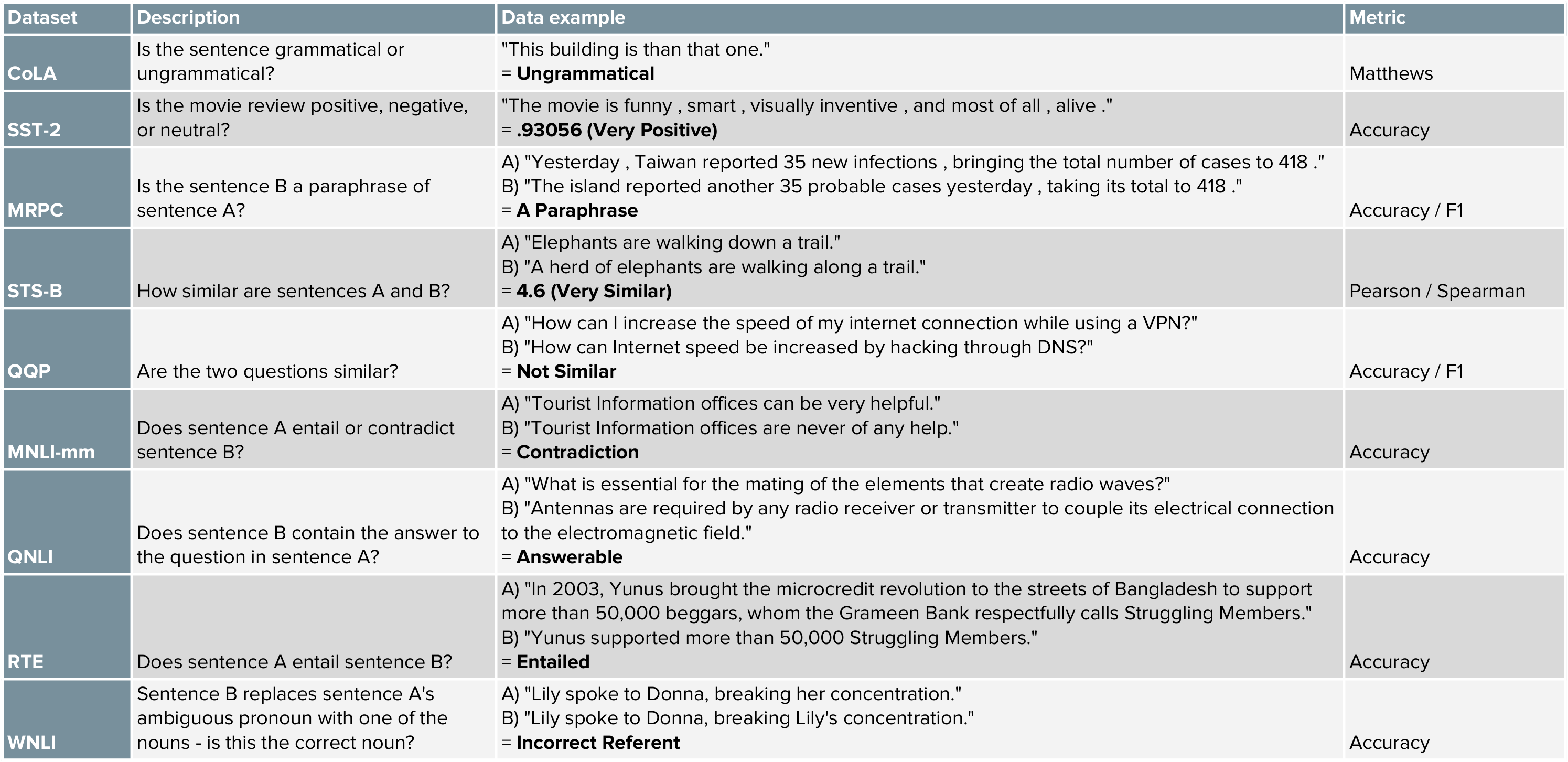taken from https://mccormickml.com A nice topping is that GLUE also provides a leaderboard with a human benchmark. So the models can compete against each other and a human benchmark. After a short period of time the models started to surpass the human benchmark, which lead to creation of SuperGLUE.

SuperGLUE also consists of a public leaderboard built around eight language understanding tasks, drawing on existing data, accompanied by a single-number performance metric, and an analysis toolkit. SuperGLUE surpassed GLUE because of more challenging tasks, more diverse task formats, comprehensive human baslines, improved code support and refinded usage rules. The following figure gives a short summary of the SuperGLUE tasks.

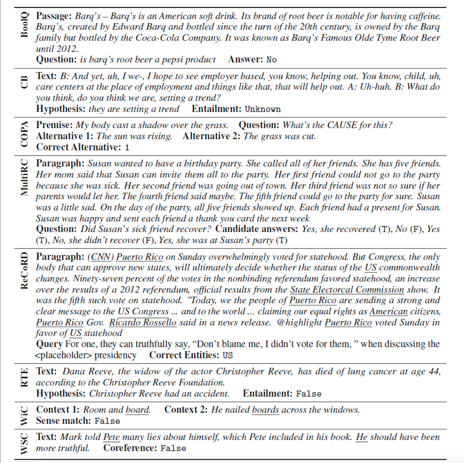
taken from https://mccormickml.com

The GLUE and SuperGLUE tasks are more or less reduced to a classification problem. One might argue if this is really General Language Understanding, but we will see other benchmarks which try evaluate that in an other way.

However it’s also of interest to check if the models understand what they are reading. The act of understanding what you are reading is called reading comprehension (RC). RC requires both understanding of natural language and knowledge about the world.

2.3.3.1.2 Stanford Question Answering Dataset (SQuAD) (1.0 & 2.0)

Rajpurkar et al. (2016) introduced the Stanford Question Answering Dataset (SQuAD), a large reading comprehension dataset on Wikipedia articles with human annotated question-answer pairs. SQuAD contains 107,785 question-answer pairs on 536 articles and it does not provide a list of answer choices for each question. The model must select the answer from all possible spans in the passage, thus needing to cope with a fairly large number of candidates. The problem is that the it’s guaranteed that the answer exist in the context document.

To address this weakness Rajpurkar, Jia, and Liang (2018) presented SQuAD 2.0, the latest version of SQuAD. SQuAD 2.0 combines existing SQuAD data with over 50,000 unanswerable questions written adversarially by crowdworkers to look similar to answerable ones.

Rajpurkar, Jia, and Liang (2018) contribution to NLP is not that they provide a deeper glimpse into the workings of QA systems, they also facilitated the creation of more non-English datasets. Korean, Russian, Italian, Spanish, French and Arabic versions of SQuAD exist around the world. XQuAD, MLQA and TyDi are multilingual question-answering datasets. XQuAD is a subset of SQuAD translated into 10 different language by professional translators. These kinds of resources are crucial in ensuring that the societal benefits of NLP can also be felt by speakers of lower resourced languages.

2.3.3.1.3 Beyond the Imitation Game Benchmark (BIG-bench)

The mentioned ones are rather old compared to Beyond the Imitation Game Benchmark (BIG-bench) (Srivastava et al. 2022). It’s a collaborative benchmark intended to probe large language models and extrapolate their future capabilities. BIG-bench already contains more than 200 tasks. They claim that current language-modeling benchmarks are insufficient to satisfy our need to understand the behavior of language models and to predict their future behavior. They mainly provide three reasons for that. One of them is the short useful lifespans. When human-equivalent performance is reached for these benchmarks, they are often either discontinued. One might call this “challenge-solve-and-replace” evaluation dynamic.

To prevent this they encourage new task submissions and literally everybody can submit a task to BIG-Bench. So they call BIG-bench a living benchmark. The review of the tasks is based on ten criteria. It includes for example “Justification”. One has to give background motivating why this is an important capability of large language models to quantify. With the inclusion of small tasks they want to improve the diversity of topics covered and enable domain experts to contribute tasks without the difficulties of distributed human labeling.

Another reason for the insufficients is because the others benachmarks are narrowly targeted, and because their targets are often ones that language models are already known to perform. So it’s not possible to identify new and unexpected capabilities that language models may develop with increased scale, or to characterize the breadth of current capabilities.

Finally, many current benchmarks use data collected through human labeling that is not performed by experts or by the task authors. Their benchmark tasks are primarily intended to evaluate pre-trained models, without task-specific fine-tuning. By focusing on such tasks in the zero- and few-shot evaluation setting, it becomes possible to provide meaningful scores for even those tasks with a very small number of examples.

The “everybody can submit” strategy also leads to inclusion a variety of tasks covering non-English languages. Till now the large language models, like GPT-3 and PaLM, perform poorly on BIG-bench relative to expert humans, which is maybe a good sign for the future. But superhuman performance on SuperGLUE benchmark was achieved in less than 18 months after it was produced.

2.3.3.1.4 WMT

There is a family of datasets which is the most popular datasets used to benchmark machine translation systems. Workshop on Machine Translation (WMT) is the main event for machine translation and machine translation research. This conference is held annually. WMT includes competitions on different aspects of machine translation. These competitions are known as shared tasks. Typically, the task organisers provide datasets and instructions. Then teams can submit their output of their models. The submissions are ranked with human evaluation.

Most of the models are evaluated on bi-lingual translation like English-to-German, but there are also tri-linguar tasks like using English to improve Russian-to-Chinese machine translation. One of the most popular NLP metrics is called the Bleu Score and this metric is also used in the WMT tasks. It is based on the idea that the closer the predicted sentence is to the human-generated target sentence, the better it is. Bleu Scores are between 0 and 1, but a score of 0.6 or 0.7 is considered the best you can achieve.

Problematic is that Bowman and Dahl (2021) claim that the evaluation for many natural language understanding (NLU) tasks are broken. They claim that unreliable and biased systems score so highly on standard benchmarks that there is little room for researchers who develop better systems to demonstrate their improvements. They provide four criteria to handle this:

Good performance on the benchmark should imply robust in-domain performance on the task
Benchmark examples should be accurately and unambiguously annotated
Benchmarks should offer adequate statistical power
Benchmarks should reveal plausibly harmful social biases in systems, and should not incentivize the creation of biased systems

Building new benchmarks that improve upon these four axes is likely to be quite difficult.

2.3.3.1.5 CheckList

Inspired by principles of behavioral testing in software engineering, Ribeiro et al. (2020) introduced CheckList, a model-agnostic and task-agnostic methodology for testing NLP models. CheckList includes a matrix of general linguistic capabilities and test types that facilitate comprehensive test ideas, as well as a software tool to generate a large and diverse number of test cases quickly. To break down potential capability failures into specific behaviors, CheckList introduces three different test types. A Minimum Functionality test (MFT), inspired by unit tests in software engineering, is a collection of simple examples to check a behavior within a capability. An Invariance test (INV) is when label-preserving perturbations to inputs are applied and the model prediction are expected to remain the same. A Directional Expectation test (DIR) is similar, except that the label is expected to change in a certain way.

Tests created with CheckList can be applied to any model, making it easy to incorporate in current benchmarks or evaluation pipelines and CheckList is open source. Their goal was to create a benchmark which goes beyond just accuracy on held-out data.

2.3.3.2 Computer Vision Benchmarks

CV models try to answer visual tasks. A visual task is a task which can be solved only by visual input. Often visual task can be solved as a binary classification problem, which is called image classification, but there are also numerous other applications for CV. This chapter will focus on image classification, semantic segmentation and object detection with their usual benchmarks datasets.

2.3.3.2.1 ImageNet Versions

It’s not only common to pre-train your model on ImageNet datasets it’s also common to benchmark the models on them. There are many different variants of ImageNet. There is ImageNet-R, a version with non-natural images such as art, cartoons and sketches, or ImageNet-A, which is a a more challenging version because they use adversarial images (Ian J Goodfellow, Shlens, and Szegedy 2014), or ImageNet-V2 (Recht et al. 2019). The last was created to check whether there is an over-fitting on the classic pre-training ImageNet dataset. They followed the creation process of the original dataset and tested to what extent current classification models generalize to new data. Recht et al. (2019) found accuracy drops for all models and suggested that these drops are not caused by adaptivity, but by the models’ inability to generalize to slightly “harder” images than those found in the original test sets.

The goal of image classification is to classify the image by assigning a label. Typically, Image Classification refers to images in which only one object appears. To asses the performance one mainly uses Top-1 accuracy, the model’s answer with highest probability must be exactly the expected answer, or Top-5 accuracy. Top-5 accuracy means that any of five highest probability answers must match the expected answer. Beyer et al. (2020) tried to answer the question “Are we done with ImageNet?” in their paper. Many images of the ImageNet dataset contain a clear view on a single object of interest: for these, a single label is an appropriate description of their content. However many other images contain multiple, similarly prominent objects, limiting the relevance of a single label (Beyer et al. 2020). In these cases, the ImageNet label is just one of many equally valid descriptions of the image and as a result an image classifier can be penalized for producing a correct description that happens to not coincide with that chosen by the ImageNet label.

In short a single label per image is not sufficient in many cases. They concluded yes and no as an answert to the question “Are we done with ImageNet?”. The shortcomings of ImageNet labels and their accuracy were identified and they provided a new ImageNet validation set ReaL (Beyer et al. 2020) (“Reassessed Labels”) and also a new metric, called ReaL accuracy (Beyer et al. 2020). The ReaL accuracy measures the precision of the model’s top-1 prediction, which is deemed correct if it is included in the set of labels. these findings suggested that although the original set of labels may be nearing the end of their useful life, ImageNet and its ReaL labels can readily benchmark progress in visual recognition for the foreseeable future.

An addition of a localization tasks to the classification tasks results into object detection. It is used to analyze more realistic cases, like mentioned above, in which multiple objects may or may not exist in an image. The location of an object is typically represented by a bounding box.

2.3.3.2.2 MS-COCO & Object365

In the recent years, the Microsoft COCO dataset or the Object365 data have become the standards to evaluate object detection algorithms, but it’s also possible to use a ImageNet dataset. The primary challenge metric is called mean Average Precision (mAP) at Intersection over Union (IoU) $=$.50:.05:.95. The IoU is the intersection of the predicted and ground truth boxes divided by the union of the predicted and ground truth boxes. IoU, also called Jaccard Index, values range from 0 to 1. Where 0 means no overlap and 1 means perfect overlap. But how is precision captured in the context of object detection? Precision is known as the ratio of $True~Positive/(True~Positive+False~Positive)$. With the help of the IoU threshold, it’s possible to decide whether the prediction is True Positive(TP), False Positive(FP), or False Negative(FN). The example below shows predictions with IoU threshold ɑ set at 0.5.

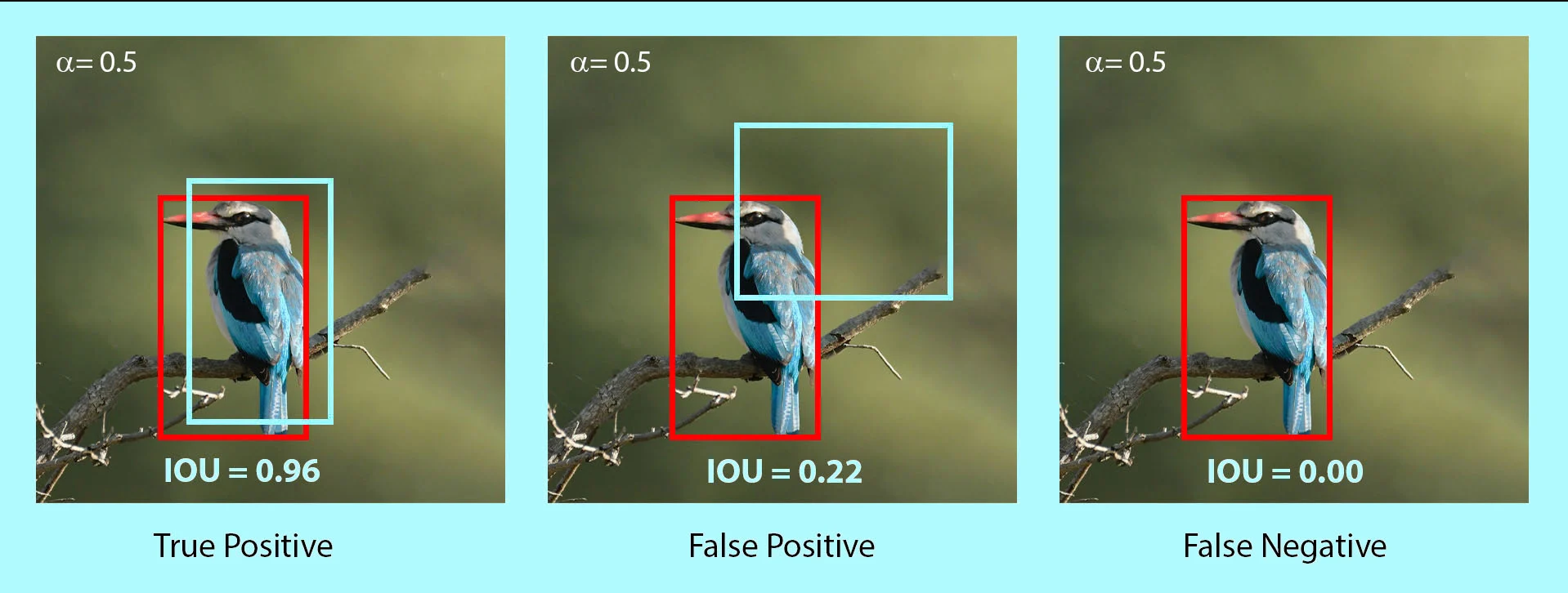taken from https://learnopencv.com The .50:.05:.95 means that one uses 10 IoU thresholds of $\{0.50, 0.55, 0.60, \dots ,0.95\}$. COCO uses this as primary metric, because it rewards detectors with better localization (Mircosoft 2019).

Object detection and image segmentation are both tasks which are concerned with localizing objects of interest in an image, but in contrast to object detection image segmentation focuses on pixel-level grouping of different semantics.

Image segmentation can be splitted into various tasks including instance segmentation, panoptic segmentation, and semantic segmentation. Instance segmentation is a task that requires the identification and segmentation of individual instance in an image. Semantic segmentation is a task that requires segmenting all the pixels in the image based on their class label. Panoptic segmentation is a combination of semantic and instance segmentation. The task is to classify all the pixels belonging to a class label, but also identify what instance of class they belong to. Panoptic and instance segmentation is often done on COCO.

2.3.3.2.3 ADE20k

Semantic segmentation can be done one ADE20K(Zhou et al. 2017). ADE are the first three letters of the name Adela Barriuso, who single handedly annotated the entire dataset and 20K is a reference to being roughly 20,000 images in the dataset. This dataset shows a high annotation complexity, because any image in ADE20K contains at least five objects, and the maximum number of object instances per image reaches 273. To asses the performance of a model on the ADE20K dataset one uses the mean IoU. It indicates the IoU between the predicted and ground-truth pixels, averaged over all the classes.

In contrast to the object detection task, the definition of TP, FP, and FN is slightly different as it is not based on a predefined threshold. TP is now the area of intersection between Ground Truth and segmentation mask. FP is the predicted area outside the Ground Truth. FN is the number of pixels in the Ground Truth area that the model failed to predict. The calculation of IoU is the same as in object detection tasks. It’s the intersection of the predicted and ground truth boxes aka. TP divided by the union of the predicted and ground truth boxes, which is essentially $TP + FN + FP$. A example is shown down below.

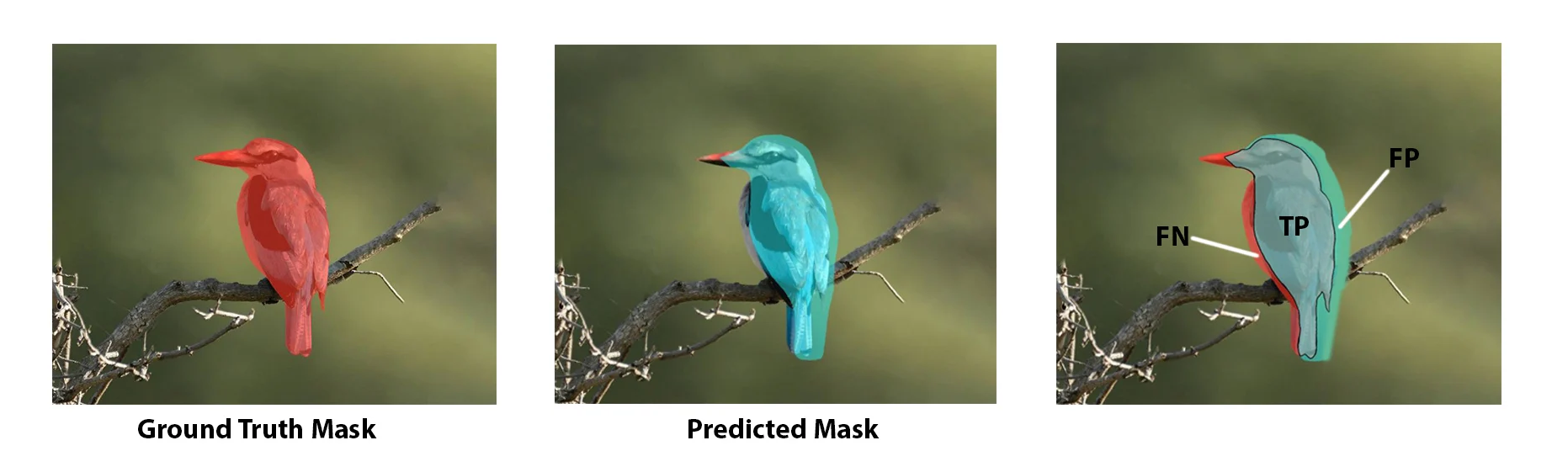
taken from https://learnopencv.com

2.3.3.3 Multi-Modal Benchmarks

Visual understanding goes well beyond object recognition or semantic segmentation. With one glance at an image, a human can effortlessly imagine the world beyond the pixels. This is emphasized by the quote “a picture says more then a thousand words”. High-order of cognition and commonsense reasoning about the world is required to infer people’s actions, goals, and mental states. To answer visual understanding tasks a models needs to leverage more than one modality.

2.3.3.3.1 Visual Commonsense Reasoning (VCR)

Visual understanding tasks require seamless integration between recognition and cognition and this task can be formalize as Visual Commonsense Reasoning (VCR). Zellers et al. (2019) introduce a new dataset called VCR. It consists of 290k multiple choice QA problems derived from 110k movie scenes. The key recipe for generating non-trivial and high-quality problems at scale is Adversarial Matching. Incorrect choices are obtained via maximum-weight bipartite matching between queries and responses. This matching transforms rich annotations into multiple choice questions with minimal bias. VCR casted as a four-way multiple choice task.

The underlying scenes come from the Large Scale Movie Description Challenge and YouTube movie clips and they searched for interesting an diverse situations to ensure this they trained and applied an “interestingnes filter”. The most interesting images were passed to Workers of Amazon Mechanical Turk. Additional context in form of video caption was given to the worker. After reading this they had to propose one to three questions about the image. For each question, they had to provide a reasonable answer and a rationale. This results is an underlying dataset with high agreement and diversity of reasoning. Almost every answer and rationale is unique. To make these cognition-level questions simple to ask, and to avoid the clunkiness of referring expressions, VCR’s language integrates object tags ([person2]) and explicitly excludes referring expressions (‘the woman on the right.’). These object tags are detected from Mask-RCNN. The following types of questions are in the benchmarks: 38% Explanation (‘Why is [person11] wearing sunglasses inside?’), 24% Activity (’What are [person1] and person[2] doing?“), 13% Temporal (”What will [person6] do after unpacking the groceries?"), 8% Mental, 7% Role, 5% Scene, 5% Hypothetical.

So in this setup, a model is provided a question, and has to pick the best answer out of four choices. Only one of the four is correct. If the model answered correctly a new question, along with the correct answer, is provided. Now the model has to justify it by picking the best rationale out of four choices. The first part is called Question Answering ($Q\rightarrow A$) and the second part Answer Justification ($QA\rightarrow R$). They combine both parts into a $Q\rightarrow AR$ metric, in which a model only gets a question right if it answers correctly and picks the right rationale. If it gets either the answer or the rationale wrong, the entire prediction will be wrong. Models are evaluated in terms of accuracy.

The results at the release were that humans find VCR easy (over 90% accuracy), and state-of-the-art vision models struggle (∼45%). At the moment of writing, the best model achieves 85.5 in ($Q\rightarrow A$), 87.5 in ($QA\rightarrow R$) and 74.9 in $Q\rightarrow AR$. So the models are closing the gap but VCR is still far from solved. An “simpler” approach to evaluate vision-language models is to ask questions without reasoning about an image.

2.3.3.3.2 Visual Question Answering 1.0 & 2.0 (VQA)

For this reason Antol et al. (2015) created an open-ended answering task and a multiple-choice task. Their dataset contains roughly 250k images, 760k questions, and 10M answers. 204k images are taken from the MS COCO dataset but also newly created created datasets are used. Three questions were collected for each image or scene. Each question was answered by ten subjects along with their confidence. The dataset contains over 760K questions with around 10M answers. “what”-, “how”-, “is”- questions are mainly used in the benchmark. But they had major flaws in their creation. An model which blindly answering “yes” without reading the rest of the question or looking at the associated image results in a VQA accuracy of 87% or the most common sport answer “tennis” was the correct answer for 41% of the questions starting with “What sport is”, and “2” is the correct answer for 39% of the questions starting with “How many” (Antol et al. 2015).

P. Zhang et al. (2016) pointed out a particular ‘visual priming bias’ in the VQA dataset. P. Zhang et al. (2016) showed that language provides a strong prior that can result in good superficial performance, without the underlying models truly understanding the visual content. P. Zhang et al. (2016) collected a balanced dataset containing pairs of complementary scenes to reduce or eliminate the strong prior of the language. Goyal et al. (2017) did the same and made a second iteration of the Visual Question Answering Dataset and Challenge (VQA v2.0). Goyal et al. (2017) balanced the popular VQA dataset (Antol et al. 2015) by collecting complementary images such that every question in balanced dataset is associated with not just a single image, but rather a pair of similar images that result in two different answers to the question. The dataset is by construction more balanced than the original VQA dataset and has approximately twice the number of image-question pairs.

2.3.3.4 GQA

Hudson and Manning (2019) introduced the GQA dataset for real-world visual reasoning and compositional question answering. It consists of 113K images and 22M questions of assorted types and varying compositionality degrees, measuring performance on an array of reasoning skills such as object and attribute recognition, transitive relation tracking, spatial reasoning, logical inference and comparisons. They also proposed Consistency, Validity and Plausibility as new measures to get more insight into models’ behavior and performance. Consistency measures responses consistency across different questions. To achieve a high consistency a model may require deeper understanding of the question semantics in context of the image. The validity metric checks whether a given answer is in the question scope, e.g. responding some color to a color question. The plausibility score goes a step further, measuring whether the answer is reasonable, or makes sense, given the question (e.g. elephant usually do not eat pizza).

They even made a comparison between GQA and VQA 2.0. They came to the conclusion that the questions of GQA are objective, unambiguous, more compositional and can be answered from the images only, potentially making this benchmark more controlled and convenient for making research progress on. Conversely, VQA questions tend to be a bit more ambiguous and subjective, at times with no clear and conclusive answer. Finally, we can see that GQA provides more questions for each image and thus covers it more thoroughly than VQA.

2.3.3.4.1 Generative Benchmarks

Almost everybody is talking right now about generative models like DALL-E2, Imagen, Parti. It seems like every month a new one is presented. But how can we compare these models? Automatic image quality and automatic image-text alignment are two reasonable evaluation metrics. Fréchet Inception Distance (FID) can be used as primary automated metric for measuring image quality. The Frechet Inception Distance compares the distribution of generated images with the distribution of real images that were used to train the generator. A small value is wanted, as it’s a distance measure. Text-image fit can be captured through automated captioning evaluation. For this an image output by the model is captioned with a model, which is able to do image captioning. The similarity of the input prompt and the generated caption is then assessed via BLEU, CIDEr, METEOR and SPICE and also human evaluation is done. Here different generative models are used with the same prompts and the human is asked to choose which output is a higher quality image and which is a better match to the input prompt. One always has to keep in mind, that the images of the generative models are always “cherry picked”. They do not typically represent, for example, a single shot interaction in which the model directly produces such an image. To make this clear, J. Yu, Xu, Koh, et al. (2022 a) showed their way of growing the cherry tree.

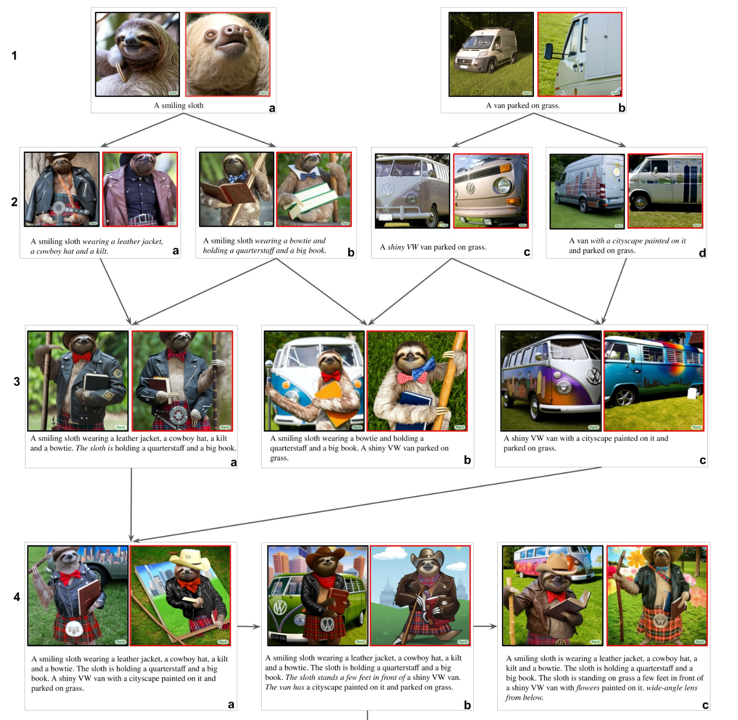
taken from Parti Paper

2.3.3.4.2 PartiPrompts, DrawBench, Localized Narratives

In a sense, this is a form of model whispering as one stretches such models to their limits. Besides to that they also present PartiPrompts (P2) which is a set of over 1600 (English) prompts curated to measure model capabilities across a variety of categories and controlled dimensions of difficulty. P2 prompts can be simple, but can also be complex, such as 67-word description they created for Vincent van Gogh’s The Starry Night. DrawBench is a similar dataset. Also the Localized Narratives dataset from the dataset section consists of long prompts and though it can also be used as a benchmark for generative models.

Current benchmarks give a good perspective on model performance on a wide range of V&L tasks, but the field is only starting to assess why models perform so well and whether models learn specific capabilities that span multiple V&L tasks.

2.3.3.4.3 FOIL it!

Shekhar et al. (2017) proposed an automatic method for creating a large dataset of real images with minimal language bias and some diagnostic abilities. They extended the MS-COCO dataset and created FOIL-COCO. FOIL stands for “Find One mismatch between Image and Language caption” and consists of images associated with incorrect captions. The captions are produced by introducing one single error (or ‘foil’) per caption in existing, human-annotated data. So each datapoint FOIL-COCO can be described as triplet consisting of an image, original and foil caption. Their data generation process consists of four main steps:

Generation of replacement word pairs
Splitting of replacement pairs into training and testing
Generation of foil captions
Mining the hardest foil caption for each image

The models are evaluated on three different tasks. The first one is Correct vs. foil classification. Given an image and a caption, the model is asked to mark whether the caption is correct or wrong. The aim is to understand whether LaVi models can spot mismatches between their coarse representations of language and visual input. The second task is Foil word detection. Given an image and a foil caption, the model has to detect the foil word. The aim is to evaluate the understanding of the system at the word level. The last task Foil word correction. Given an image, a foil caption and the foil word, the model has to detect the foil and provide its correction. The aim is to check whether the system’s visual representation is fine-grained enough to be able to extract the information necessary to correct the error. Their hypothesis is that systems which, like humans, deeply integrate the language and vision modalities, should spot foil captions quite easily.

2.3.3.4.4 VALSE

Vision And Language Structured Evaluation (VALSE) (Parcalabescu et al. 2022) builds on the same idea. This benchmark aims to gauge the sensitivity of pre-trained V&L models to foiled instances. They coverd a wide spectrum of basic linguistic phenomena affecting the linguistic and visual modalities: existence, plurality, counting, spatial relations, actions, and entity coreference. To generate the foils they first use strong language models to propose foil and second they use natural language inference to filter out captions that still can describe the image. To do this in an automatic fashion they use the image as an premise and the caption its entailed hypothesis. Additionally they use the captian as an premise and the foil as the hypothesis. If an NLI model predicts the foil to be neutral or a contradiction with respect to the caption, they see this as an indicator for a good foil. At last the used human annotators to validate all generated testing data. Mainly the MS-COCO dataset is used. VALSE is as a task-independent, zero-shot benchmark to assess the extent to which models learn to ground specific linguistic phenomena as a consequence of their pretraining.

2.3.3.5 Other Benchmarks

As we don’t live in a world with unlimited resources, it’s also important to keep track of how much energy is consumed to train the models and how big the carbon footprint is. Strubell, Ganesh, and McCallum (2019 b) investigated some NLP models and benchmarked model training and development costs in terms of dollars and estimated $CO_2$ emissions. They came to the result that training a single BERT base model without hyperparameter tuning on GPUs requires the same energy as a trans-American flight. On average a human is responsible for 5t $CO_2$ per year and Strubell, Ganesh, and McCallum (2019 b) estimated that the training procedure of a big Transformer with neural architecture search emitted 284t of $CO_2$. Works (Lottick et al. 2019, @henderson2020towards) have released online tools to benchmark their energy usage and initiatives such as the SustainNLP workshop have since taken up the goal of prioritizing computationally efficient hardware and algorithms. These findings are just some points one should keep in mind.

In the following chapters we will see how the multimodal architectures use these datasets and also how they perform on the given benchmarks.

References

Antol, Stanislaw, Aishwarya Agrawal, Jiasen Lu, Margaret Mitchell, Dhruv Batra, C Lawrence Zitnick, and Devi Parikh. 2015. “Vqa: Visual Question Answering.” In Proceedings of the Ieee International Conference on Computer Vision, 2425–33.

Bahdanau, Dzmitry, Kyunghyun Cho, and Yoshua Bengio. 2014. “Neural Machine Translation by Jointly Learning to Align and Translate.” http://arxiv.org/abs/1409.0473.

Bandy, Jack, and Nicholas Vincent. 2021. “Addressing" Documentation Debt" in Machine Learning Research: A Retrospective Datasheet for Bookcorpus.” arXiv Preprint arXiv:2105.05241.

Bender, Emily M., Timnit Gebru, Angelina McMillan-Major, and Shmargaret Shmitchell. 2021. “On the Dangers of Stochastic Parrots: Can Language Models Be Too Big?” In Proceedings of the 2021 Acm Conference on Fairness, Accountability, and Transparency, 610–23. FAccT ’21. Virtual Event, Canada: Association for Computing Machinery. https://doi.org/10.1145/3442188.3445922.

Beyer, Lucas, Olivier J Hénaff, Alexander Kolesnikov, Xiaohua Zhai, and Aäron van den Oord. 2020. “Are We Done with Imagenet?” arXiv Preprint arXiv:2006.07159.

Birhane, Abeba, Vinay Uday Prabhu, and Emmanuel Kahembwe. 2021. “Multimodal Datasets: Misogyny, Pornography, and Malignant Stereotypes.” arXiv Preprint arXiv:2110.01963.

Bojanowski, Piotr, Edouard Grave, Armand Joulin, and Tomas Mikolov. 2016. “Enriching Word Vectors with Subword Information.” http://arxiv.org/abs/1607.04606.

Bowman, Samuel R, and George E Dahl. 2021. “What Will It Take to Fix Benchmarking in Natural Language Understanding?” arXiv Preprint arXiv:2104.02145.

Bromley, Jane, Isabelle Guyon, Yann LeCun, Eduard Säckinger, and Roopak Shah. 1993. “Signature Verification Using a" Siamese" Time Delay Neural Network.” Advances in Neural Information Processing Systems 6.

Brown, Tom, Benjamin Mann, Nick Ryder, Melanie Subbiah, Jared D Kaplan, Prafulla Dhariwal, Arvind Neelakantan, et al. 2020. “Language Models Are Few-Shot Learners.” Advances in Neural Information Processing Systems 33: 1877–1901.

Caron, Mathilde, Ishan Misra, Julien Mairal, Priya Goyal, Piotr Bojanowski, and Armand Joulin. 2020. “Unsupervised Learning of Visual Features by Contrasting Cluster Assignments.” CoRR. https://arxiv.org/abs/2006.09882.

Chen, Ting, Simon Kornblith, Mohammad Norouzi, and Geoffrey Hinton. 2020a. “A Simple Framework for Contrastive Learning of Visual Representations.” arXiv. https://doi.org/10.48550/ARXIV.2002.05709.

Cho, Kyunghyun, Bart van Merrienboer, Caglar Gulcehre, Dzmitry Bahdanau, Fethi Bougares, Holger Schwenk, and Yoshua Bengio. 2014. “Learning Phrase Representations Using Rnn Encoder-Decoder for Statistical Machine Translation.” http://arxiv.org/abs/1406.1078.

Clark, Kevin, Urvashi Khandelwal, Omer Levy, and Christopher D. Manning. 2019. “What Does Bert Look at? An Analysis of Bert’s Attention.” http://arxiv.org/abs/1906.04341.

Da, Jeff, and Jungo Kasai. 2019. “Cracking the Contextual Commonsense Code: Understanding Commonsense Reasoning Aptitude of Deep Contextual Representations.” http://arxiv.org/abs/1910.01157.

Deng, Jia, Wei Dong, Richard Socher, Li-Jia Li, Kai Li, and Li Fei-Fei. 2009. “Imagenet: A Large-Scale Hierarchical Image Database.” In 2009 Ieee Conference on Computer Vision and Pattern Recognition, 248–55. Ieee.

Devlin, Jacob, Ming-Wei Chang, Kenton Lee, and Kristina Toutanova. 2018b. “BERT: Pre-Training of Deep Bidirectional Transformers for Language Understanding.” http://arxiv.org/abs/1810.04805.

Dhamala, Jwala, Tony Sun, Varun Kumar, Satyapriya Krishna, Yada Pruksachatkun, Kai-Wei Chang, and Rahul Gupta. 2021. “Bold: Dataset and Metrics for Measuring Biases in Open-Ended Language Generation.” In Proceedings of the 2021 Acm Conference on Fairness, Accountability, and Transparency, 862–72.

Dosovitskiy, Alexey, Lucas Beyer, Alexander Kolesnikov, Dirk Weissenborn, Xiaohua Zhai, Thomas Unterthiner, Mostafa Dehghani, et al. 2020. “An Image Is Worth 16x16 Words: Transformers for Image Recognition at Scale.” arXiv Preprint arXiv:2010.11929.

Dosovitskiy, Alexey, Lucas Beyer, Alexander Kolesnikov, Dirk Weissenborn, Xiaohua Zhai, Thomas Unterthiner, Mostafa Dehghani, et al. 2020a. “An Image Is Worth 16x16 Words: Transformers for Image Recognition at Scale.” CoRR. https://arxiv.org/abs/2010.11929.

Dosovitskiy, Alexey, Lucas Beyer, Alexander Kolesnikov, Dirk Weissenborn, Xiaohua Zhai, Thomas Unterthiner, Mostafa Dehghani, et al. 2020b. “An Image Is Worth 16x16 Words: Transformers for Image Recognition at Scale.” CoRR abs/2010.11929. https://arxiv.org/abs/2010.11929.

Dwibedi, Debidatta, Yusuf Aytar, Jonathan Tompson, Pierre Sermanet, and Andrew Zisserman. 2021. “With a Little Help from My Friends: Nearest-Neighbor Contrastive Learning of Visual Representations.” CoRR abs/2104.14548. https://arxiv.org/abs/2104.14548.

Education, IBM Cloud. 2020a. “What Is Supervised Learning?” www.ibm.com.

Education, IBM Cloud. 2020b. “What Is Unsupervised Learning?” www.ibm.com.

Ettinger, Allyson. 2019. “What Bert Is Not: Lessons from a New Suite of Psycholinguistic Diagnostics for Language Models.” http://arxiv.org/abs/1907.13528.

Fellbaum, Christiane. 2010. “WordNet.” In Theory and Applications of Ontology: Computer Applications, 231–43. Springer.

Forbes, Maxwell, Ari Holtzman, and Yejin Choi. 2019. “Do Neural Language Representations Learn Physical Commonsense?” http://arxiv.org/abs/1908.02899.

Gao, Jiyang, Zhen Li, Ram Nevatia, and others. 2017. “Knowledge Concentration: Learning 100k Object Classifiers in a Single Cnn.” arXiv Preprint arXiv:1711.07607.

Gao, Leo, Stella Biderman, Sid Black, Laurence Golding, Travis Hoppe, Charles Foster, Jason Phang, et al. 2020. “The Pile: An 800gb Dataset of Diverse Text for Language Modeling.” arXiv Preprint arXiv:2101.00027.

Gokaslan, Aaron, and Vanya Cohen. 2019. “OpenWebText Corpus.”

Goodfellow, Ian J, Jonathon Shlens, and Christian Szegedy. 2014. “Explaining and Harnessing Adversarial Examples.” arXiv Preprint arXiv:1412.6572.

Google. 2022. “Embeddings: Translating to a Lower-Dimensional Space.”

Goyal, Yash, Tejas Khot, Douglas Summers-Stay, Dhruv Batra, and Devi Parikh. 2017. “Making the V in Vqa Matter: Elevating the Role of Image Understanding in Visual Question Answering.” In Proceedings of the Ieee Conference on Computer Vision and Pattern Recognition, 6904–13.

Grill, Jean-Bastien, Florian Strub, Florent Altch’e, Corentin Tallec, Pierre H. Richemond, Elena Buchatskaya, Carl Doersch, et al. 2020. “Bootstrap Your Own Latent: A New Approach to Self-Supervised Learning.” Neurips.

Grill, Jean-Bastien, Florian Strub, Florent Altché, Corentin Tallec, Pierre H. Richemond, Elena Buchatskaya, Carl Doersch, et al. 2020. “Bootstrap Your Own Latent: A New Approach to Self-Supervised Learning.” arXiv. https://doi.org/10.48550/ARXIV.2006.07733.

Guo, Yandong, Lei Zhang, Yuxiao Hu, Xiaodong He, and Jianfeng Gao. 2016. “Ms-Celeb-1m: A Dataset and Benchmark for Large-Scale Face Recognition.” In European Conference on Computer Vision, 87–102. Springer.

Hart, B., and T. R. Risley. 1995. “Meaningful Differences in the Everyday Experience of Young American Children.” Baltimore, MD: Paul H. Brookes Publishing Company,

He, Kaiming, Xinlei Chen, Saining Xie, Yanghao Li, Piotr Dollár, and Ross Girshick. 2022. “Masked Autoencoders Are Scalable Vision Learners.” In Proceedings of the Ieee/Cvf Conference on Computer Vision and Pattern Recognition, 16000–16009.

He, Kaiming, Xiangyu Zhang, Shaoqing Ren, and Jian Sun. 2015. “Deep Residual Learning for Image Recognition.” CoRR. http://arxiv.org/abs/1512.03385.

Hinton, Geoffrey, Oriol Vinyals, Jeff Dean, and others. 2015. “Distilling the Knowledge in a Neural Network.” arXiv Preprint arXiv:1503.02531 2 (7).

Howard, Andrew G., Menglong Zhu, Bo Chen, Dmitry Kalenichenko, Weijun Wang, Tobias Weyand, Marco Andreetto, and Hartwig Adam. 2017. “MobileNets: Efficient Convolutional Neural Networks for Mobile Vision Applications.” CoRR abs/1704.04861. http://arxiv.org/abs/1704.04861.

Huang, Yanping, Yonglong Cheng, Dehao Chen, HyoukJoong Lee, Jiquan Ngiam, Quoc V. Le, and Zhifeng Chen. 2018. “GPipe: Efficient Training of Giant Neural Networks Using Pipeline Parallelism.” CoRR abs/1811.06965. http://arxiv.org/abs/1811.06965.

Hudson, Drew A, and Christopher D Manning. 2019. “Gqa: A New Dataset for Real-World Visual Reasoning and Compositional Question Answering.” In Proceedings of the Ieee/Cvf Conference on Computer Vision and Pattern Recognition, 6700–6709.

Jaspreet. 2019. “A Concise History of Neural Networks by Jaspreet Towards Data Science.” towardsdatascience.com.

Jia, Chao, Yinfei Yang, Ye Xia, Yi-Ting Chen, Zarana Parekh, Hieu Pham, Quoc Le, Yun-Hsuan Sung, Zhen Li, and Tom Duerig. 2021a. “Scaling up Visual and Vision-Language Representation Learning with Noisy Text Supervision.” In International Conference on Machine Learning, 4904–16. PMLR.

Joseph, K. J., Salman H. Khan, Fahad Shahbaz Khan, and Vineeth N. Balasubramanian. 2021. “Towards Open World Object Detection.” CoRR abs/2103.02603. https://arxiv.org/abs/2103.02603.

Jumper, John, Richard Evans, Alexander Pritzel, Tim Green, Michael Figurnov, Olaf Ronneberger, Kathryn Tunyasuvunakool, et al. 2021. “Highly Accurate Protein Structure Prediction with AlphaFold.” Nature 596 (7873): 583–89. https://doi.org/10.1038/s41586-021-03819-2.

Koehn, Philipp. 2005. “Europarl: A Parallel Corpus for Statistical Machine Translation.” In Proceedings of Machine Translation Summit X: Papers, 79–86.

Kolesnikov, Alexander, Lucas Beyer, Xiaohua Zhai, Joan Puigcerver, Jessica Yung, Sylvain Gelly, and Neil Houlsby. 2019. “Large Scale Learning of General Visual Representations for Transfer.” arXiv Preprint arXiv:1912.11370 2 (8).

Krishna, Ranjay, Yuke Zhu, Oliver Groth, Justin Johnson, Kenji Hata, Joshua Kravitz, Stephanie Chen, et al. 2017. “Visual Genome: Connecting Language and Vision Using Crowdsourced Dense Image Annotations.” International Journal of Computer Vision 123 (1): 32–73.

Krizhevsky, Alex, Geoffrey Hinton, and others. 2009. “Learning Multiple Layers of Features from Tiny Images.”

Krizhevsky, Alex, Ilya Sutskever, and Geoffrey E Hinton. 2012a. “ImageNet Classification with Deep Convolutional Neural Networks.” In Advances in Neural Information Processing Systems, edited by F. Pereira, C. J. Burges, L. Bottou, and K. Q. Weinberger. Vol. 25. Curran Associates, Inc. https://proceedings.neurips.cc/paper/2012/file/c399862d3b9d6b76c8436e924a68c45b-Paper.pdf.

Kuznetsova, Alina, Hassan Rom, Neil Alldrin, Jasper Uijlings, Ivan Krasin, Jordi Pont-Tuset, Shahab Kamali, et al. 2020. “The Open Images Dataset V4.” International Journal of Computer Vision 128 (7): 1956–81.

Lialin, Vladislav, Kevin Zhao, Namrata Shivagunde, and Anna Rumshisky. 2022. “Life After Bert: What Do Other Muppets Understand About Language?” http://arxiv.org/abs/2205.10696.

Lin, Tsung-Yi, Michael Maire, Serge Belongie, James Hays, Pietro Perona, Deva Ramanan, Piotr Dollár, and C Lawrence Zitnick. 2014a. “Microsoft Coco: Common Objects in Context.” In European Conference on Computer Vision, 740–55. Springer.

Lin, Yongjie, Yi Chern Tan, and Robert Frank. 2019. “Open Sesame: Getting Inside BERT’s Linguistic Knowledge.” In Proceedings of the 2019 ACL Workshop BlackboxNLP: Analyzing and Interpreting Neural Networks for NLP. Association for Computational Linguistics. https://doi.org/10.18653/v1/w19-4825.

Lottick, Kadan, Silvia Susai, Sorelle A Friedler, and Jonathan P Wilson. 2019. “Energy Usage Reports: Environmental Awareness as Part of Algorithmic Accountability.” arXiv Preprint arXiv:1911.08354.

Mahajan, Dhruv, Ross Girshick, Vignesh Ramanathan, Kaiming He, Manohar Paluri, Yixuan Li, Ashwin Bharambe, and Laurens Van Der Maaten. 2018. “Exploring the Limits of Weakly Supervised Pretraining.” In Proceedings of the European Conference on Computer Vision (Eccv), 181–96.

Manning, Chris, Anna Goldie, and John Hewitt. 2022. “Stanford Cs224n: Natural Language Processing with Deep Learning.”

Mayer, Thomas, and Michael Cysouw. 2014. “Creating a Massively Parallel Bible Corpus.” Oceania 135 (273): 40.

MICHAEL BARTHEL, JESSE HOLCOMB, GALEN STOCKING, and AMY MITCHELL. 2016. “Reddit News Users More Likely to Be Male, Young and Digital in Their News Preferences.” 2016. https://www.pewresearch.org/journalism/2016/02/25/reddit-news-users-more-likely-to-be-male-young-and-digital-in-their-news-preferences/.

Mikolov, Tomas, Kai Chen, Greg Corrado, and Jeffrey Dean. 2013a. “Efficient Estimation of Word Representations in Vector Space.” arXiv Preprint arXiv:1301.3781.

Mikolov, Tomas, Quoc V. Le, and Ilya Sutskever. 2013. “Exploiting Similarities Among Languages for Machine Translation.” http://arxiv.org/abs/1309.4168.

Mikolov, Tomas, Ilya Sutskever, Kai Chen, Greg Corrado, and Jeffrey Dean. 2013. “Distributed Representations of Words and Phrases and Their Compositionality.” http://arxiv.org/abs/1310.4546.

Mineault, Patrick. 2021. “Unsupervised Models of the Brain.” 2021. https://xcorr.net/2021/12/31/2021-in-review-unsupervised-brain-models/.

Mircosoft. 2019. “Evaluate:Detection.” 2019. https://cocodataset.org/#detection-eval.

“Neural Networks - History.” 2022. cs.stanford.edu.

Parcalabescu, Letitia, Michele Cafagna, Lilitta Muradjan, Anette Frank, Iacer Calixto, and Albert Gatt. 2022. “VALSE: A Task-Independent Benchmark for Vision and Language Models Centered on Linguistic Phenomena.” In Proceedings of the 60th Annual Meeting of the Association for Computational Linguistics (Volume 1: Long Papers), 8253–80. Association for Computational Linguistics. https://aclanthology.org/2022.acl-long.567.

Perez, Ethan, Douwe Kiela, and Kyunghyun Cho. 2021a. “True Few-Shot Learning with Language Models.” http://arxiv.org/abs/2105.11447.

Pilehvar, Mohammad Taher, and Jose Camacho-Collados. 2021. Embeddings in Natural Language Processing. Springer International Publishing. https://doi.org/10.1007/978-3-031-02177-0.

Pont-Tuset, Jordi, Jasper Uijlings, Soravit Changpinyo, Radu Soricut, and Vittorio Ferrari. 2020. “Connecting Vision and Language with Localized Narratives.” In European Conference on Computer Vision, 647–64. Springer.

Prabhu, Vinay Uday, and Abeba Birhane. 2020. “Large Image Datasets: A Pyrrhic Win for Computer Vision?” arXiv Preprint arXiv:2006.16923.

Radford, Alec, Jong Wook Kim, Chris Hallacy, Aditya Ramesh, Gabriel Goh, Sandhini Agarwal, Girish Sastry, et al. 2021. “Learning Transferable Visual Models from Natural Language Supervision.” In International Conference on Machine Learning, 8748–63. PMLR.

Radford, Alec, Karthik Narasimhan, Tim Salimans, and Ilya Sutskever. 2018. “Improving Language Understanding by Generative Pre-Training.”

Raffel, Colin, Noam Shazeer, Adam Roberts, Katherine Lee, Sharan Narang, Michael Matena, Yanqi Zhou, Wei Li, and Peter J. Liu. 2019a. “Exploring the Limits of Transfer Learning with a Unified Text-to-Text Transformer.” http://arxiv.org/abs/1910.10683.

Raghu, Maithra, Ben Poole, Jon Kleinberg, Surya Ganguli, and Jascha Sohl-Dickstein. 2016. “On the Expressive Power of Deep Neural Networks.” arXiv. https://doi.org/10.48550/ARXIV.1606.05336.

Rajpurkar, Pranav, Robin Jia, and Percy Liang. 2018. “Know What You Don’t Know: Unanswerable Questions for Squad.” arXiv Preprint arXiv:1806.03822.

Rajpurkar, Pranav, Jian Zhang, Konstantin Lopyrev, and Percy Liang. 2016. “Squad: 100,000+ Questions for Machine Comprehension of Text.” arXiv Preprint arXiv:1606.05250.

Ramachandran, Prajit, Niki Parmar, Ashish Vaswani, Irwan Bello, Anselm Levskaya, and Jonathon Shlens. 2019. “Stand-Alone Self-Attention in Vision Models.” CoRR abs/1906.05909. http://arxiv.org/abs/1906.05909.

Recht, Benjamin, Rebecca Roelofs, Ludwig Schmidt, and Vaishaal Shankar. 2019. “Do Imagenet Classifiers Generalize to Imagenet?” In International Conference on Machine Learning, 5389–5400. PMLR.

Ribeiro, Marco Tulio, Tongshuang Wu, Carlos Guestrin, and Sameer Singh. 2020. “Beyond Accuracy: Behavioral Testing of Nlp Models with Checklist.” arXiv Preprint arXiv:2005.04118.

Ritchie, Hannah, Max Roser, and Pablo Rosado. 2020. “$CO_2$ And Greenhouse Gas Emissions.” Our World in Data.

Rosset, Corby. 2020. “Turing-Nlg: A 17-Billion-Parameter Language Model by Microsoft.” Microsoft Blog 1 (2).

Saharia, Chitwan, William Chan, Saurabh Saxena, Lala Li, Jay Whang, Emily Denton, Seyed Kamyar Seyed Ghasemipour, et al. 2022a. “Photorealistic Text-to-Image Diffusion Models with Deep Language Understanding.” arXiv Preprint arXiv: Arxiv-2205.11487.

Saifee, Moiz. 2020. “GPT-3: The New Mighty Language Model from Openai.”

Schick, Timo, and Hinrich Schütze. 2020. “Exploiting Cloze Questions for Few Shot Text Classification and Natural Language Inference.” http://arxiv.org/abs/2001.07676.

Schuhmann, Christoph, Richard Vencu, Romain Beaumont, Robert Kaczmarczyk, Clayton Mullis, Aarush Katta, Theo Coombes, Jenia Jitsev, and Aran Komatsuzaki. 2021a. “Laion-400m: Open Dataset of Clip-Filtered 400 Million Image-Text Pairs.” arXiv Preprint arXiv:2111.02114.

Sejnowski, Terrence J. 2020. “The Unreasonable Effectiveness of Deep Learning in Artificial Intelligence.” Proceedings of the National Academy of Sciences U.S.A. (2020) Https://Www.pnas.org/Content/Early/2020/01/23/1907373117. https://doi.org/10.1073/pnas.1907373117.

Shah, Deval. 2022. “Self-Supervised Learning and Its Applications - Neptune.ai.” neptune.ai.

Shao, Shuai, Zeming Li, Tianyuan Zhang, Chao Peng, Gang Yu, Xiangyu Zhang, Jing Li, and Jian Sun. 2019. “Objects365: A Large-Scale, High-Quality Dataset for Object Detection.” In Proceedings of the Ieee/Cvf International Conference on Computer Vision, 8430–9.

Shekhar, Ravi, Sandro Pezzelle, Yauhen Klimovich, Aurélie Herbelot, Moin Nabi, Enver Sangineto, and Raffaella Bernardi. 2017. “Foil It! Find One Mismatch Between Image and Language Caption.” arXiv Preprint arXiv:1705.01359.

Sheng, Emily, Kai-Wei Chang, Premkumar Natarajan, and Nanyun Peng. 2019. “The Woman Worked as a Babysitter: On Biases in Language Generation.” arXiv Preprint arXiv:1909.01326.

Simonyan, Karen, and Andrew Zisserman. 2014. “Very deep convolutional networks for large-scale image recognition.” arXiv Preprint arXiv:1409.1556.

Srinivasan, Krishna, Karthik Raman, Jiecao Chen, Michael Bendersky, and Marc Najork. 2021. “Wit: Wikipedia-Based Image Text Dataset for Multimodal Multilingual Machine Learning.” In Proceedings of the 44th International Acm Sigir Conference on Research and Development in Information Retrieval, 2443–9.

Srivastava, Aarohi, Abhinav Rastogi, Abhishek Rao, Abu Awal Md Shoeb, Abubakar Abid, Adam Fisch, Adam R Brown, et al. 2022. “Beyond the Imitation Game: Quantifying and Extrapolating the Capabilities of Language Models.” arXiv Preprint arXiv:2206.04615.

Strubell, Emma, Ananya Ganesh, and Andrew McCallum. 2019a. “Energy and Policy Considerations for Deep Learning in NLP.” In Proceedings of the 57th Annual Meeting of the Association for Computational Linguistics, 3645–50. Florence, Italy: Association for Computational Linguistics. https://doi.org/10.18653/v1/P19-1355.

Strubell, Emma, Ananya Ganesh, and Andrew McCallum. 2019b. “Energy and Policy Considerations for Deep Learning in Nlp.” arXiv Preprint arXiv:1906.02243.

Sun, Chen, Abhinav Shrivastava, Saurabh Singh, and Abhinav Gupta. 2017. “Revisiting Unreasonable Effectiveness of Data in Deep Learning Era.” In Proceedings of the Ieee International Conference on Computer Vision, 843–52.

Sutskever, Ilya, Oriol Vinyals, and Quoc V. Le. 2014. “Sequence to Sequence Learning with Neural Networks.” http://arxiv.org/abs/1409.3215.

Tan, Mingxing, and Quoc V. Le. 2019a. “EfficientNet: Rethinking Model Scaling for Convolutional Neural Networks.” https://doi.org/10.48550/ARXIV.1905.11946.

Tan, Mingxing, and Quoc V. 2019b. “EfficientNet: Rethinking Model Scaling for Convolutional Neural Networks.” CoRR abs/1905.11946. http://arxiv.org/abs/1905.11946.

techslang. 2020. “What Is Self-Supervised Learning? — Definition by Techslang.” www.techslang.com.

Tiu, Ekin. 2021. “Understanding Contrastive Learning by Ekin Tiu Towards Data Science.” towardsdatascience.com.

Torralba, Antonio, and Alexei A Efros. 2011. “Unbiased Look at Dataset Bias.” In CVPR 2011, 1521–8. IEEE.

Vaswani, Ashish, Noam Shazeer, Niki Parmar, Jakob Uszkoreit, Llion Jones, Aidan N. Gomez, Lukasz Kaiser, and Illia Polosukhin. 2017a. “Attention Is All You Need.” http://arxiv.org/abs/1706.03762.

Vaswani, Ashish, Noam Shazeer, Niki Parmar, Jakob Uszkoreit, Llion Jones, Aidan N Gomez, Łukasz Kaiser, and Illia Polosukhin. 2017b. “Attention Is All You Need.” Advances in Neural Information Processing Systems 30.

Voita, Elena, David Talbot, Fedor Moiseev, Rico Sennrich, and Ivan Titov. 2019. “Analyzing Multi-Head Self-Attention: Specialized Heads Do the Heavy Lifting, the Rest Can Be Pruned.” http://arxiv.org/abs/1905.09418.

Wang, Jun, and Shengchen Li. 2018. “Detection and Classification of Acoustic Scenes and Events 2018 Self-Attention Mechanism Based System for Dcase2018 Challenge Task1 and Task4,” August. https://doi.org/10.13140/RG.2.2.28317.13281.

Website. 2020. “Localized Narratives Data and Visualization.” 2020. https://google.github.io/localized-narratives.

Wenzek, Guillaume, Marie-Anne Lachaux, Alexis Conneau, Vishrav Chaudhary, Francisco Guzmán, Armand Joulin, and Edouard Grave. 2019. “Ccnet: Extracting High Quality Monolingual Datasets from Web Crawl Data.” arXiv Preprint arXiv:1911.00359.

Xie, Qizhe, Eduard H. Hovy, Minh-Thang Luong, and Quoc V. Le. 2019. “Self-Training with Noisy Student Improves Imagenet Classification.” CoRR abs/1911.04252. http://arxiv.org/abs/1911.04252.

Xue, Linting, Noah Constant, Adam Roberts, Mihir Kale, Rami Al-Rfou, Aditya Siddhant, Aditya Barua, and Colin Raffel. 2020. “MT5: A Massively Multilingual Pre-Trained Text-to-Text Transformer.” arXiv Preprint arXiv:2010.11934.

Yann, Lecun, and Misra Ishan. 2021. “Self-Supervised Learning: The Dark Matter of Intelligence.” 2021. https://ai.facebook.com/blog/self-supervised-learning-the-dark-matter-of-intelligence/.

Young, Peter, Alice Lai, Micah Hodosh, and Julia Hockenmaier. 2014. “From Image Descriptions to Visual Denotations: New Similarity Metrics for Semantic Inference over Event Descriptions.” Transactions of the Association for Computational Linguistics 2: 67–78.

Yu, Jiahui, Yuanzhong Xu, Jing Koh, Thang Luong, Gunjan Baid, Vijay Vasudevan, Alexander Ku, et al. 2022a. “Scaling Autoregressive Models for Content-Rich Text-to-Image Generation.” https://doi.org/10.48550/arXiv.2206.10789.

Yuan, Sha, Zhao Shuai, Leng Jiahong, Xue Zhao, Zhao Hanyu, and Tang Jie. 2022. “WuDaoMM: A Large-Scale Multi-Modal Dataset for Pre-Training Models.” arXiv Preprint arXiv:2203.11480.

Zagoruyko, Sergey, and Nikos Komodakis. 2016. “Wide Residual Networks.” CoRR abs/1605.07146. http://arxiv.org/abs/1605.07146.

Zellers, Rowan, Yonatan Bisk, Ali Farhadi, and Yejin Choi. 2019. “From Recognition to Cognition: Visual Commonsense Reasoning.” In Proceedings of the Ieee/Cvf Conference on Computer Vision and Pattern Recognition, 6720–31.

Zhang, Peng, Yash Goyal, Douglas Summers-Stay, Dhruv Batra, and Devi Parikh. 2016. “Yin and Yang: Balancing and Answering Binary Visual Questions.” In Proceedings of the Ieee Conference on Computer Vision and Pattern Recognition, 5014–22.

Zhou, Bolei, Hang Zhao, Xavier Puig, Sanja Fidler, Adela Barriuso, and Antonio Torralba. 2017. “Scene Parsing Through Ade20k Dataset.” In Proceedings of the Ieee Conference on Computer Vision and Pattern Recognition, 633–41.

Zhou, Yanqi, Sudip Roy, Amirali Abdolrashidi, Daniel Wong, Peter Ma, Qiumin Xu, Hanxiao Liu, et al. 2020. “Transferable Graph Optimizers for Ml Compilers.” NeurIPS 2020. http://arxiv.org/abs/2010.12438.

Zhu, Yukun, Ryan Kiros, Rich Zemel, Ruslan Salakhutdinov, Raquel Urtasun, Antonio Torralba, and Sanja Fidler. 2015. “Aligning Books and Movies: Towards Story-Like Visual Explanations by Watching Movies and Reading Books.” In Proceedings of the Ieee International Conference on Computer Vision, 19–27.

Zhuang, Chengxu, Siming Yan, Aran Nayebi, Martin Schrimpf, Michael C Frank, James J DiCarlo, and Daniel LK Yamins. 2021. “Unsupervised Neural Network Models of the Ventral Visual Stream.” Proceedings of the National Academy of Sciences 118 (3): e2014196118.