Multi-Fidelity
An introduction to multi-fidelity is given in J. E. Fieldsend and R. M. Everson, The Rolling Tide Evolutionary Algorithm: A Multiobjective Optimizer for Noisy Optimization Problems. In its current state, mosmafs supports two ways of performing multi-fidelity optimization: Selected by generation, and selected by dominance. Multi-fidelity by generation is simply performed by changing the fidelity of the objective function after a given number of generations. Multi-fidelity by dominance is performed by evaluating a point with low fidelity first, and then enabling high fidelity if the first evaluation suggests that the point is not dominated by any previous result.
Preparation
This vignette starts where the previous vignette leaves off and expects the following preparation:
devtools::install_github("jakobbossek/ecr2")
library("ecr")
library("magrittr")
library("ggplot2")
library("ParamHelpers")
library("mlr")
library("mlrCPO")
library("mosmafs")
task.whole <- create.hypersphere.data(3, 2000) %>%
  create.classif.task(id = "sphere") %>%
  task.add.permuted.cols(10)
rows.whole <- sample(2000)
task <- subsetTask(task.whole, rows.whole[1:500])
task.hout <- subsetTask(task.whole, rows.whole[501:2000])

lrn <- makeLearner("classif.rpart", maxsurrogate = 0)

ps.simple <- pSS(
  maxdepth: integer[1, 30],
  minsplit: integer[2, 30],
  cp: numeric[0.001, 0.999])

fitness.fun.simple <- makeObjective(lrn, task, ps.simple, cv5,
  holdout.data = task.hout)

ps.objective <- getParamSet(fitness.fun.simple)

mutator.simple <- combine.operators(ps.objective,
  numeric = ecr::setup(mutGauss, sdev = 0.1),
  integer = ecr::setup(mutGaussInt, sdev = 3),
  selector.selection = mutBitflipCHW)

crossover.simple <- combine.operators(ps.objective,
  numeric = recPCrossover,
  integer = recPCrossover,
  selector.selection = recPCrossover)

initials <- sampleValues(ps.objective, 32, discrete.names = TRUE)
Fidelity Argument
An objective function optimized with slickEcr() may have a fidelity argument which should choose the fidelity at which the function is evaluated. It can take any numeric value chosen (at another point) by the user, but it should make sense to take a weighted mean of results by this fidelity:
(obj(x, fidelity = a) * a + obj(x, fidelity = b) * b) / (a + b)A sensible usage of fidelity is to choose the number of resampling iterations through it.
The makeObjective() function will create a multi-fidelity compatible objective function if its resampling argument is a function, mapping from numeric(1) to a resampling object. The results for different fidelities should usually not be subsets of one another, because the evaluation for different fidelities is sometimes averaged over, which can lead to over-emphasis of some resampling folds.
nRes <- function(n) {
  makeResampleDesc("Subsample", split = 0.9, iters = n)
}
We can use this function to create a multi-fidelity fitness function:
fitness.fun <- makeObjective(lrn, task, ps.simple, nRes, holdout.data = task.hout)

formals(fitness.fun)
#> $args
#>
#>
#> $fidelity
#> NULL
#>
#> $holdout
#> [1] FALSE
Generation-Wise Multi-Fidelity
The slickEcr() function accepts the fidelity argument, which must be a data.frame with two or three columns. For generation-wise multi-fidelity, we give it a data.frame with two columns, with the first column indicating the generation at which a certain fidelity should be used, and the second column containing the fidelity to use. To use fidelity 1 for the first five generations, then fidelity 3, for another five generations, and finally 5 for the last five, the data.frame would be
fidelity <- data.frame(
    c(1, 6, 11),
    c(1, 3, 5))
print(fidelity)
#>   c.1..6..11. c.1..3..5.
#> 1           1          1
#> 2           6          3
#> 3          11          5
This is given to slickEcr():
run.gen.mufi <- slickEcr(
    fitness.fun = fitness.fun,
    lambda = 16,
    population = initials,
    mutator = mutator.simple,
    recombinator = crossover.simple,
    generations = 15,
    fidelity = fidelity)
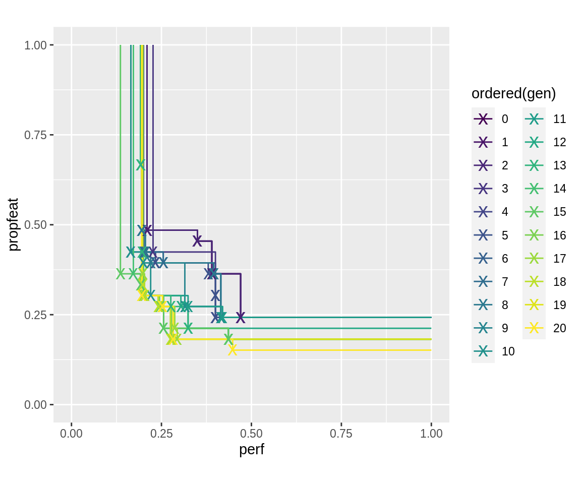
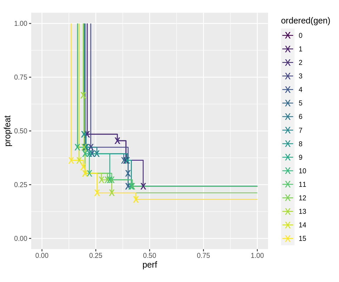
The plot of resulting pareto-fronts notably has later generation’s pareto fronts seemingly dominated by individuals from earlier generations. This is because in the log-object, the fitness of the first generations was evaluated using the low fidelity of these generations. In later generations, these points were re-evaluated using the larger fidelity.
plot_fronts <- function(run) {
  fronts <- fitnesses(run, function(x) paretoEdges(x, c(1, 1)))
  ggplot(data = fronts, aes(x = perf, y = propfeat, color = ordered(gen))) +
    geom_line() +
    geom_point(data = fronts[fronts$point, ], shape = "x", size = 5) +
    xlim(0, 1) +
    ylim(0, 1) +
    coord_fixed()
}

plot_fronts(run.gen.mufi)
The fidelity that was used for each individuum can be extracted from its "fidelity" attribute. It can be accessed using the attr() method or the popAggregate() utility function. The runtime will scale approximately linearly (with an added constant overhead) in this case. The sum of all fidelity options used for each generation can also be inspected using the log.newinds logging object–it may represent a proxy for the computational ressources that were used. Note how the generations with changing fidelity are present twice: for re-evaluation with new fidelity, and for ordinary evaluation of new individuals.
populations <- getPopulations(run.gen.mufi$log)

ind1.gen1 <- populations[[1]]$population[[1]]
attr(ind1.gen1, "fidelity")
#> [1] 1
attr(ind1.gen1, "runtime")
#>    elapsed
#> 0.09976384

ind1.gen7 <- populations[[7]]$population[[1]]
attr(ind1.gen7, "fidelity")
#> [1] 2
attr(ind1.gen7, "runtime")
#>  elapsed
#> 0.126887

ind1.gen15 <- populations[[15]]$population[[1]]
attr(ind1.gen15, "fidelity")
#> [1] 3
attr(ind1.gen15, "runtime")
#>   elapsed
#> 0.1533511

getStatistics(run.gen.mufi$log.newinds)
#>    gen runtime.mean runtime.sum fidelity.sum size      population
#> 1    0   0.10083978    3.226873           32   32            init
#> 2    1   0.10273623    1.643780           16   16       offspring
#> 3    2   0.10331556    1.653049           16   16       offspring
#> 4    3   0.10844688    1.735150           16   16       offspring
#> 5    4   0.09916852    1.586696           16   16       offspring
#> 6    5   0.09887493    1.581999           16   16       offspring
#> 7    6   0.14354162    4.593332           64   32 fidelity.reeval
#> 8    6   0.13711842    2.193895           32   16       offspring
#> 9    7   0.15008382    2.401341           32   16       offspring
#> 10   8   0.13176804    2.108289           32   16       offspring
#> 11   9   0.12631964    2.021114           32   16       offspring
#> 12  10   0.14509410    2.321506           32   16       offspring
#> 13  11   0.18596968    5.951030           96   32 fidelity.reeval
#> 14  11   0.17461410    2.793826           48   16       offspring
#> 15  12   0.16876434    2.700230           48   16       offspring
#> 16  13   0.16680493    2.668879           48   16       offspring
#> 17  14   0.16426940    2.628310           48   16       offspring
#> 18  15   0.17184141    2.749462           48   16       offspring
The cumulative fidelity up to each generation can be computed using the collectResult() function. This makes it possible to analyse progress up to a certain point of computational expenditure.
cres <- collectResult(run.gen.mufi)
ggplot(cres, aes(x = cum.fid, y = eval.domHV, color = "Training")) +
  geom_line() + geom_point(size = 1) +
  geom_point(data = cres[cres$fid.reeval, ], shape = "x", size = 5) +
  geom_line(aes(x = cum.fid, y = true.hout.domHV, color = "Holdout")) +
  ylim(0, 1)
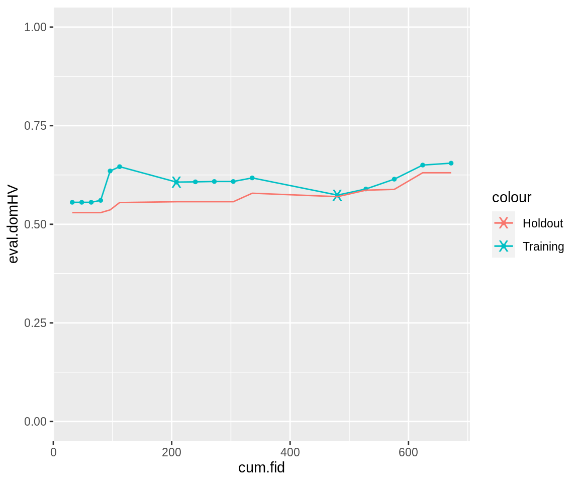
The “x” mark the points at which fidelity reevaluation occurred: There a jump downward in hypervolume is possible. Also, the plot shows a large jump in cumulative fidelity before each reevaluation, because the whole population is reevaluated at these points.
Multi-Fidelity by Dominance
The slickEcr() fidelity argument accepts data.frames with three columns in the case that different fidelity should be used for points that lie on the pareto-front than those that, in a first evaluation, are dominated. This can be combined with generation-wise multi-fidelity, but our first example will only have one row. It evaluates simple holdout-resampling for each point, and, if the result seems to be better than previous evaluations with the same number of features, re-does the resampling with ten-times repeated holdout resampling, which results in overall 11 evaluations for this point.
fidelity <- data.frame(1, 1, 10)
print(fidelity)
#>   X1 X1.1 X10
#> 1  1    1  10
run.dom.mufi <- slickEcr(
    fitness.fun = fitness.fun,
    lambda = 16,
    population = initials,
    mutator = mutator.simple,
    recombinator = crossover.simple,
    generations = 15,
    fidelity = fidelity)
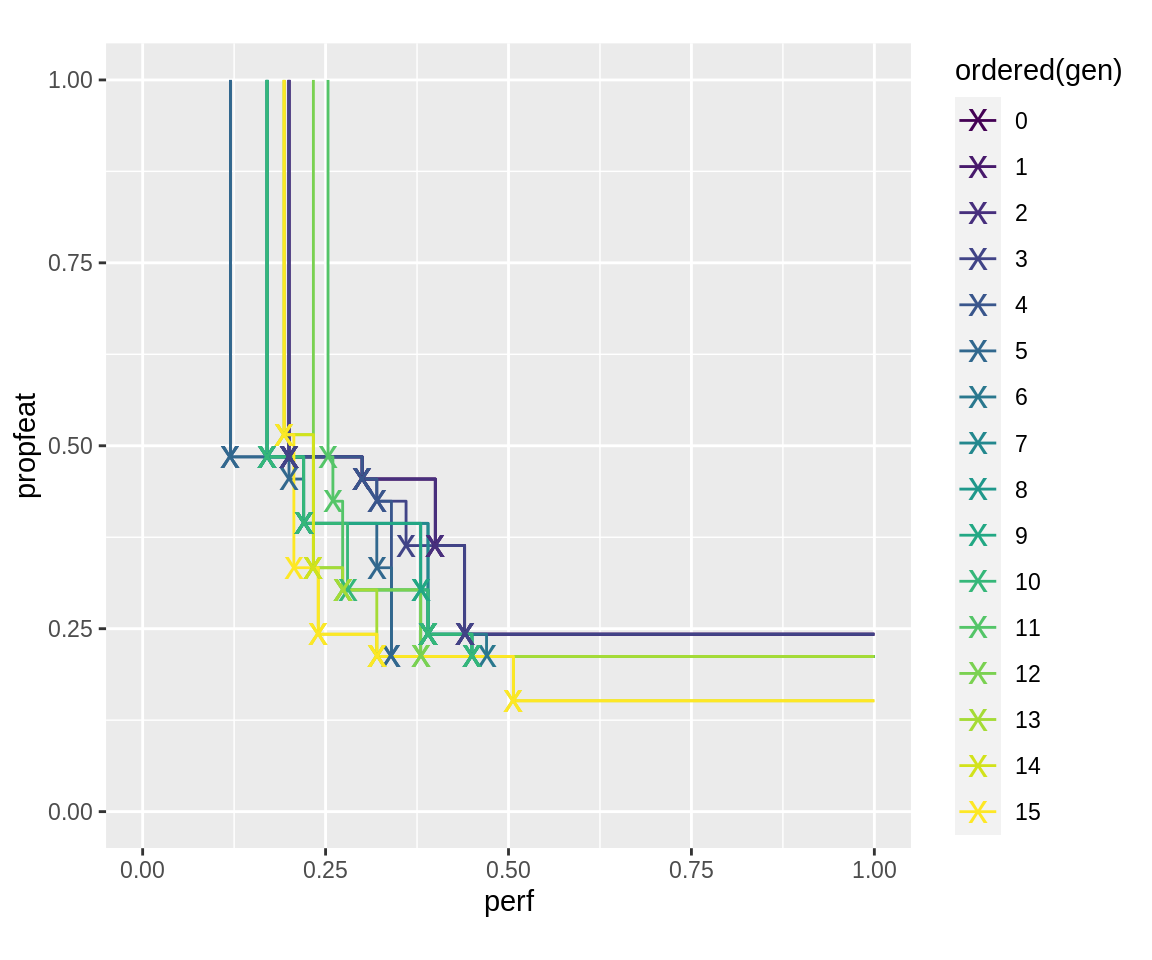
plot_fronts(run.dom.mufi)
The log.newinds object will again provide information about the aggregated runtime and fidelity used. Some generations perform more high-fidelity evaluations than others (and consequently have longer runtime).
getStatistics(run.dom.mufi$log.newinds)
#>    gen runtime.mean runtime.sum fidelity.sum size population
#> 1    0    0.1388156    4.442100           64   32       init
#> 2    1    0.1259382    2.015012           19   16  offspring
#> 3    2    0.1200721    1.921153           22   16  offspring
#> 4    3    0.1087775    1.740440           20   16  offspring
#> 5    4    0.1151526    1.842442           19   16  offspring
#> 6    5    0.1040050    1.664080           16   16  offspring
#> 7    6    0.1164272    1.862835           19   16  offspring
#> 8    7    0.1144615    1.831384           18   16  offspring
#> 9    8    0.1093364    1.749383           21   16  offspring
#> 10   9    0.1142647    1.828235           18   16  offspring
#> 11  10    0.1024632    1.639412           16   16  offspring
#> 12  11    0.1145763    1.833220           20   16  offspring
#> 13  12    0.1064261    1.702817           18   16  offspring
#> 14  13    0.1092579    1.748126           19   16  offspring
#> 15  14    0.1163302    1.861284           20   16  offspring
#> 16  15    0.1106061    1.769697           21   16  offspring
Use the popAggregate() function to get collected information about fidelity in individuals in a generation. The following shows the fidelities used in generation 2:
popAggregate(run.dom.mufi$log, "fidelity")[[2]]
#>  [1] 2 2 2 2 2 2 2 1 2 2 2 2 2 2 2 2 2 2 1 1 2 1 1 1 2 2 2 2 1 1 2 2
Note that, the fidelity is 11 for some candidates, as they were promising after one holdout resampling and were additionally reevaluated with ten-times repeated holdout resampling.
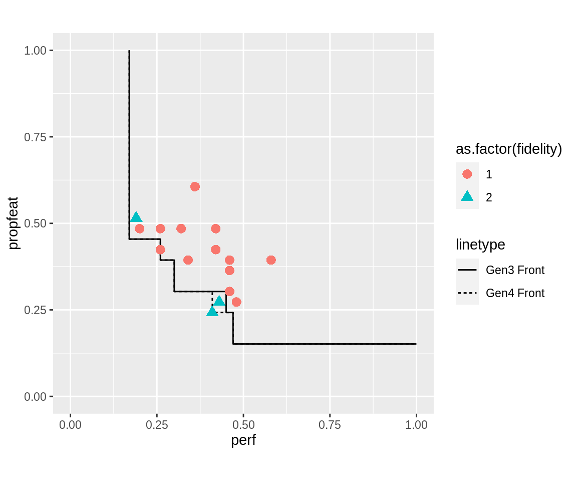
Individual evaluation fidelity can be retrieved, again, from a logged individual’s attributes. The following plots the pareto-front of generation 3, and the individuals sampled for generation 4. All individuals sampled with high fidelity lie close to the pareto-front, but some may, after high-fidelity evaluation, have turned out to actually be dominated by the old generation.
gen.i <- 3
logobj <- run.dom.mufi$log.newinds
stat <- getStatistics(logobj)
pop <- popAggregate(logobj, c("fidelity", "fitness"), data.frame = TRUE)
ngen.info <- pop[[which(stat$gen == gen.i + 1)]]
front <- fitnesses(run.dom.mufi, function(x) paretoEdges(x, c(1, 1))) %>%
    subset(gen == gen.i)
new.front <- fitnesses(run.dom.mufi, function(x) paretoEdges(x, c(1, 1))) %>%
    subset(gen == gen.i + 1)


ggplot() +
  geom_line(data = front, aes(x = perf, y = propfeat, linetype = "Gen3 Front")) +
  geom_line(data = new.front, aes(x = perf, y = propfeat, linetype = "Gen4 Front")) +
  geom_point(data = ngen.info,
    aes(x = fitness.perf, y = fitness.propfeat,
      shape = as.factor(fidelity),
      color = as.factor(fidelity),
      size = 3)) +
  scale_size_identity() +
  guides(colour = guide_legend(override.aes = list(size=3))) +
  xlim(0, 1) +
  ylim(0, 1) +
  coord_fixed()
All of the Above
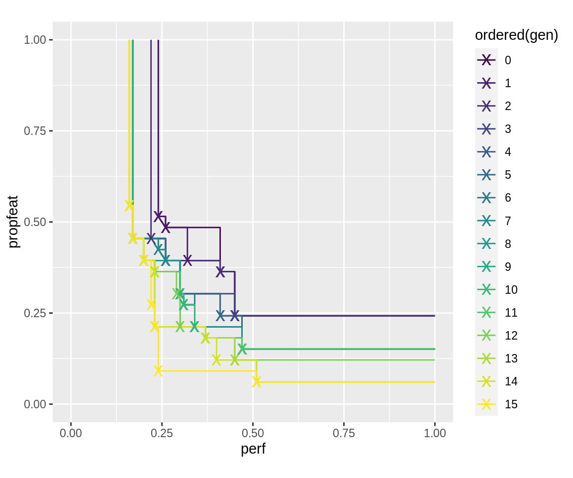
The two approaches can, of course, be combined. It should be noted that the initial generation, as well as each generation after a fidelity-jump, is evaluated with the “high” fidelity column number. The following, for example, evaluates generation 1 with fidelity 6, generation 6 with fidelity 11, and generation 11 with fidelity 15. In between, new points are evaluated with low fidelity first and then re-evaluated on high-fidelity if they seem to not be dominated by the previous generation. Because of this, fidelity-jumps tend to be relatively computationally expensive and should be done sparingly if at all. If unbiased.fidelity is set (the default), only an upward step in total fidelity of pareto set elements (i.e. sum of 2nd and 3rd column if three columns are given, otherwise just value in 2nd column) leads to a re-evaluation of all fidelity. It should be set whenever the expectation value of evaluated fitness does not change with changing fidelity between generations (note that it is strongly recommended that evaluations with the two fidelities in each row have the same or very close expectation values).
fidelity <- data.frame(
    c(1, 3, 6, 11),
    c(1, 2, 3, 5),
    c(5, 4, 8, 10))
print(fidelity)
#>   c.1..3..6..11. c.1..2..3..5. c.5..4..8..10.
#> 1              1             1              5
#> 2              3             2              4
#> 3              6             3              8
#> 4             11             5             10
run.all.mufi <- slickEcr(
    fitness.fun = fitness.fun,
    lambda = 16,
    population = initials,
    mutator = mutator.simple,
    recombinator = crossover.simple,
    generations = 15,
    fidelity = fidelity)
getStatistics(run.all.mufi$log.newinds)
#>    gen runtime.mean runtime.sum fidelity.sum size      population
#> 1    0    0.1349974    4.319916           64   32            init
#> 2    1    0.1034026    1.654441           16   16       offspring
#> 3    2    0.1027900    1.644640           18   16       offspring
#> 4    3    0.1703576    5.451442           96   32 fidelity.reeval
#> 5    3    0.1419464    2.271142           34   16       offspring
#> 6    4    0.1412301    2.259681           36   16       offspring
#> 7    5    0.1488443    2.381508           33   16       offspring
#> 8    6    0.2098481    6.715138          128   32 fidelity.reeval
#> 9    6    0.2038832    3.262132           52   16       offspring
#> 10   7    0.1713009    2.740814           48   16       offspring
#> 11   8    0.1760516    2.816825           50   16       offspring
#> 12   9    0.1874103    2.998565           51   16       offspring
#> 13  10    0.1668958    2.670333           51   16       offspring
#> 14  11    0.2317432    7.415781          160   32 fidelity.reeval
#> 15  11    0.2139883    3.423813           65   16       offspring
#> 16  12    0.2398051    3.836881           66   16       offspring
#> 17  13    0.1986673    3.178677           67   16       offspring
#> 18  14    0.2085184    3.336294           68   16       offspring
#> 19  15    0.2021234    3.233974           67   16       offspring
plot_fronts(run.all.mufi)
Run Continuation
When continuing finished runs using the continueEcr() functionality, it is possible to submit a new fidelity data.frame to change fidelity behaviour. Note that generations continue to count from where previous evaluations left off. Therefore, in the following example, the entry for generation 1 is ignored, the fidelity used for all new offspring is 20 and rises to 25.
fidelity.new <- data.frame(
    c(1, 10, 17, 19),
    c(11, 20, 23, 25))
print(fidelity.new)
#>   c.1..10..17..19. c.11..20..23..25.
#> 1                1                11
#> 2               10                20
#> 3               17                23
#> 4               19                25
run.all.mufi.20 <- continueEcr(run.all.mufi, 5,
  lambda = 8, fidelity = fidelity.new)
getStatistics(run.all.mufi.20$log.newinds)
#>    gen runtime.mean runtime.sum fidelity.sum size      population
#> 1    0    0.1406437    4.500599           64   32            init
#> 2    1    0.1082329    1.731727           16   16       offspring
#> 3    2    0.1053250    1.685200           18   16       offspring
#> 4    3    0.1651821    5.285826           96   32 fidelity.reeval
#> 5    3    0.1355341    2.168545           34   16       offspring
#> 6    4    0.1492810    2.388497           36   16       offspring
#> 7    5    0.1410677    2.257082           33   16       offspring
#> 8    6    0.2284782    7.311304          128   32 fidelity.reeval
#> 9    6    0.1781086    2.849737           52   16       offspring
#> 10   7    0.1829772    2.927636           48   16       offspring
#> 11   8    0.1821415    2.914265           50   16       offspring
#> 12   9    0.1674030    2.678448           51   16       offspring
#> 13  10    0.1850420    2.960672           51   16       offspring
#> 14  11    0.2491200    7.971839          160   32 fidelity.reeval
#> 15  11    0.2116532    3.386452           65   16       offspring
#> 16  12    0.2116322    3.386116           66   16       offspring
#> 17  13    0.2056859    3.290975           67   16       offspring
#> 18  14    0.2112479    3.379966           68   16       offspring
#> 19  15    0.2399218    3.838749           67   16       offspring
#> 20  16    0.7884217   25.229494          640   32 fidelity.reeval
#> 21  16    0.7354913    5.883931          160    8       offspring
#> 22  17    0.9127745   29.208783          736   32 fidelity.reeval
#> 23  17    0.8066059    6.452847          184    8       offspring
#> 24  18    0.8443415    6.754732          184    8       offspring
#> 25  19    0.9973229   31.914332          800   32 fidelity.reeval
#> 26  19    0.9646255    7.717004          200    8       offspring
#> 27  20    0.9145475    7.316380          200    8       offspring
plot_fronts(run.all.mufi.20)