SAILS: Surrogate-based Analysis of Interactions via Local Effect Smooths

A model-agnostic framework that detects pairwise feature interactions in a black-box model, categorizes their functional form, and visualizes them, all in a single integrated pipeline.

Timo Heiß^1,2, Julia Herbinger^3,4, Bernd Bischl^1,2, Giuseppe Casalicchio^1,2,4

¹Department of Statistics, LMU Munich ²Munich Center for Machine Learning (MCML) ³Leibniz Institute for Prevention Research and Epidemiology (BIPS), Bremen ⁴Center for Advanced Studies (CAS), LMU Munich

XKDD 2026, 8th International Workshop on eXplainable Knowledge Discovery in Data Mining at ECML PKDD 2026

Paper PDF Code BibTeX

Some methods tell you which features interact. Others visualize an interaction once you know where to look. SAILS does both, in one pipeline.

Detecting interactions and showing what they look like have largely been separate lines of work. The H-statistic and Shapley interaction indices quantify how strong an interaction is, but say nothing about its shape. The methods that do visualize interactions each stop somewhere:

Two-dimensional feature effects

2D-ALE and 2D partial dependence plots handle any interaction type, but you must know in advance which pair interacts, and contour surfaces are hard to read.

Regional effects

REPID and GADGET plot feature effects in subspaces less affected by interactions. That exposes interacting features, not the interaction form, and struggles with continuous interactions.

Integrated approaches

The closest method that both detects and visualizes interaction forms is limited to product-separable interactions, assumes independent features, and is threshold-sensitive.

SAILS runs all of this in one pipeline. It finds the interacting features, determines the form of each interaction, and plots that form, for any two-way interaction.

What SAILS produces. For a black box containing a $\sin(\pi x_1 x_3)$ interaction, the general visualization draws one curve per interval of $x_1$, each showing how the interaction effect varies with $x_3$. The sine shape is directly visible. Select intervals of $x_1$ in the list to read them one at a time; the rest stay in the background in gray.

Summary

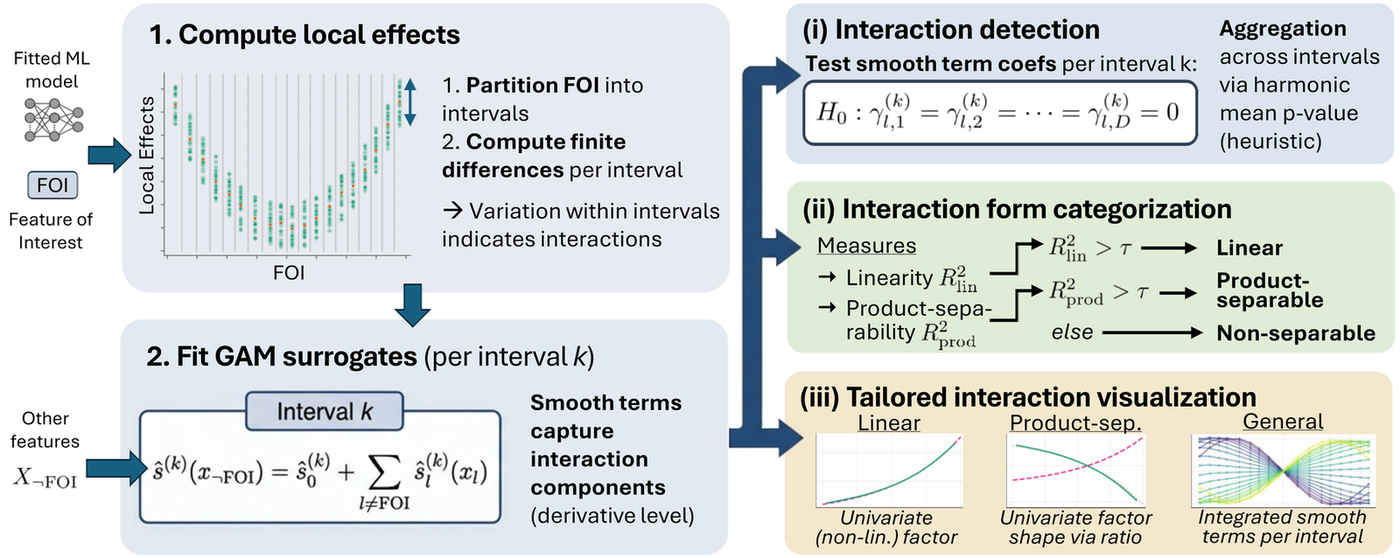
SAILS (Surrogate-based Analysis of Interactions via Local Effect Smooths) analyzes the pairwise interactions of a feature of interest (FOI) in any fitted regression model. It partitions the FOI into intervals, estimates ALE local effects there, and fits one interpretable GAM surrogate per interval to those local effects. Because local effects at a fixed FOI value can only vary through interactions involving the FOI, each smooth term of a surrogate isolates one pairwise interaction, on the level of derivatives. From these smooth terms, SAILS derives three integrated capabilities: interaction detection, categorization of the interaction form, and a visualization tailored to that form.

In controlled simulations, detection stays reliable under feature correlations and degrades only marginally under higher-order interactions. Categorization separates interaction types perfectly under two-way interactions and independence; the linearity measure is fairly robust, while the product-separability measure suffers under correlations and higher-order terms. All three visualization strategies recover the true interaction forms closely under independence and lose accuracy only gradually under moderate correlations. On a real-world power consumption task, the interactions SAILS recovers match plausible demand patterns.

Highlights

Detecting Relevant Interactions

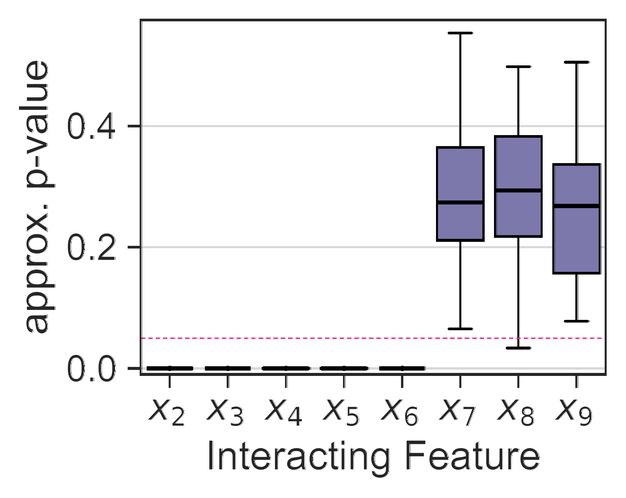
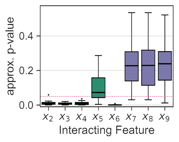
Each smooth term is tested against the null hypothesis that its basis coefficients vanish. Interval-wise p-values are aggregated with the harmonic mean p-value and corrected, yielding one value per feature to assess the "significance" of its interaction with the FOI.

Interaction Form, Not Just Strength

Every detected interaction is sorted into one of three forms: linear in the FOI, product-separable, or non-product-separable. Two $R^2$-based measures do the sorting, read off the smooth terms and their ratios, with no assumption about which form to expect.

Three Tailored Visualizations

Linear and product-separable interactions each get a single-curve plot showing how the interacting feature affects the interaction. Everything else is recovered by integrating the smooth terms. That general visualization covers any two-way interaction and is easy to understand.

Model-Agnostic and Reproducible

SAILS needs only a fitted regression model and its training data. The Python implementation works with any scikit-learn-compatible model and numerical features, and every experiment in the paper is reproducible from the repository.

How SAILS Works

Overview diagram of the SAILS framework: step 1 computes local effects by partitioning the feature of interest into intervals and taking finite differences; step 2 fits a GAM surrogate per interval; the smooth terms then feed interaction detection via a hypothesis test, interaction form categorization via the linearity and product-separability measures, and three tailored visualizations. — The SAILS pipeline: two steps (compute local effects, fit GAM surrogates) enabling three capabilities (detection, categorization, visualization).

Step 1: Local Effects in Intervals of the Feature of Interest

The FOI $X_j$ is partitioned into $K$ intervals, and for every observation the local effect is estimated by a finite difference across its interval, normalized by the interval width. Local effects are locally decomposable: they depend only on the main effect of the FOI and on the interaction components that involve it. Fixing the FOI therefore leaves interactions as the only source of variation. For $\hat{f}(\mathbf{x}) = x_1^3 + x_2 + 0.5\,x_1 x_2$, for instance, $\partial_1 \hat f = 3x_1^2 + 0.5\,x_2$, so at a fixed $x_1$ all remaining spread comes from the $0.5\,x_1x_2$ term.

Step 2: One GAM Surrogate per Interval

Within each interval $k$, SAILS fits a generalized additive model with the remaining features as inputs and the local effects as target:

$$\hat s^{(k)}(\mathbf{x}^{(i)}_{-j}) = \hat s^{(k)}_0 + \sum_{l \neq j} \hat s^{(k)}_l\big(x^{(i)}_l\big)$$

Assuming the model contains only up to two-way interactions, and building on classical results for additive model components, the paper conjectures that the fitted parts recover the FANOVA derivatives up to centering constants:

$$\hat s^{(k)}_0 \approx \partial_j g_j(\bar z_{k,j}) + c^{(k)}_0, \qquad \hat s^{(k)}_l(x_l) \approx \partial_j g_{jl}(\bar z_{k,j}, x_l) - c^{(k)}_l$$

This correspondence is a conjecture, not a theorem. The paper validates it empirically instead of proving it, and reports an in-sample goodness-of-fit check that flags surrogate misspecification from higher-order interactions.

The Three Capabilities

Every smooth term $\hat s^{(k)}_l$ is thus a picture of one pairwise interaction, at one value of the FOI, on the derivative level. All three capabilities read those terms:

i Interaction Detection Finds which features interact with the feature of interest.

The test. For every feature $X_l$ and every interval $k$, SAILS tests the smooth term against the null hypothesis that all $D$ of its basis coefficients vanish, $H_0 : \gamma^{(k)}_{l,1} = \gamma^{(k)}_{l,2} = \cdots = \gamma^{(k)}_{l,D} = 0$. Under i.i.d. Gaussian errors this is an F-test, which returns one p-value $p^{(k)}_l$ per interval.

Why the result is a heuristic. The local effects are computed directly from the fitted model with no additive noise term, so the i.i.d. error assumption does not formally hold, and the smooth terms are penalized. The values should therefore be read as a heuristic for interaction significance, not as exact p-values.

Aggregation and correction. Tests in neighboring intervals of the same feature are dependent, since a strong interaction in one interval makes significance in the next one likely. SAILS combines the interval-wise values with the harmonic mean p-value, which is robust under dependence, then applies a Benjamini-Hochberg false discovery rate correction across features.

How to read it. One value per feature. Features below a threshold $\alpha$ are flagged as interacting with the FOI, with $\alpha = 0.05$ as the default by analogy with conventional significance levels. Use the values as a flag and a ranking, not as calibrated probabilities.

ii Interaction Categorization Categorizes each detected interaction into: linear in the FOI, product-separable, or non-product-separable.

The three forms. An interaction $g_{jl}$ is linear with respect to the FOI $X_j$ when $g_{jl}(x_j, x_l) = (x_j - \mathbb{E}[X_j])\,\phi_l(x_l)$, and product-separable when $g_{jl}(x_j, x_l) = \phi_j(x_j)\,\phi_l(x_l)$, for univariate functions $\phi_j$ and $\phi_l$. Linearity is the special case $\phi_j(x_j) = x_j - \mathbb{E}[X_j]$. Everything that does not factor into a product of two univariate functions is non-product-separable, which is the general case: the effect of $x_l$ changes shape, and not only scale, as the FOI moves. Interactions such as $\sin(\pi x_j x_l)$ fall here.

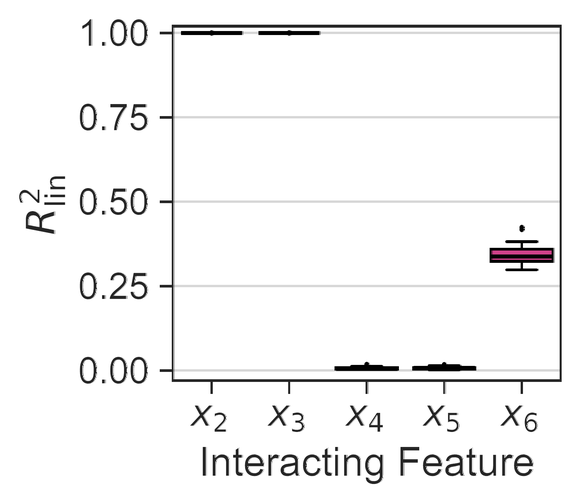
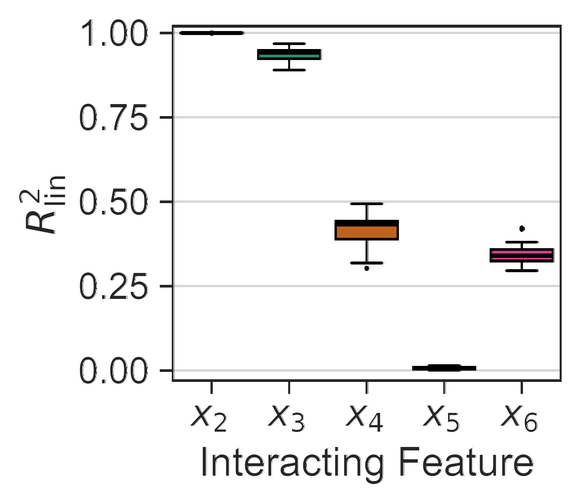
Linearity, $R^2_{\text{lin}}$. If an interaction is linear in the FOI, its derivative does not depend on the FOI, so the smooth terms of all intervals coincide. SAILS tests for that: evaluate every smooth term at interval-specific grid points, pool all evaluations, and fit a single penalized spline to them. $R^2_{\text{lin}}$ is the coefficient of determination of that fit, so it measures how well one curve, independent of the FOI, explains all smooth terms at once.

Product-separability, $R^2_{\text{prod}}$. If an interaction is product-separable, the smooth terms share one shape and differ only by a scaling factor, so dividing each by its own value at a fixed reference point $\tilde{x}^{\text{ref}}_l$ makes them coincide. SAILS reuses the same evaluations, forms those ratios, and fits a single penalized spline to the pooled ratios. $R^2_{\text{prod}}$ is the coefficient of determination of that fit.

Non-product-separability. This form has no measure of its own. If a non-product-separable interaction is present, the smooth terms differ in shape across intervals, so neither a single curve nor a single ratio curve can explain them, and both measures come out low. The category is therefore what remains once the other two are ruled out, and it is the one the general visualization exists for.

How to read them. Compare both against a threshold $\tau$, for example $\tau = 0.9$ for 90% explained variance. $R^2_{\text{lin}} \geq \tau$ means linear in the FOI; $R^2_{\text{prod}} \geq \tau$ without linearity means product-separable; below both means non-product-separable. This categorization helps to better understand the interactions and choose appropriate (potentially easier) visualization strategies.

iii Interaction Visualization Plots the interaction with one of three strategies, chosen by the categorization.

Linear interaction, when $R^2_{\text{lin}} \geq \tau$. Plot the univariate smoother that $R^2_{\text{lin}}$ was computed from. It estimates $\phi_l$, the entire dependence of the interaction on $x_l$.

A parabola opening upward, plotted against x2. The dashed reference curve for 2x2 squared and the solid SAILS curve lie on top of each other. — The $x_1 \times x_2$ interaction of $\hat f(\mathbf{x}) = 3x_1 + 2x_1x_2^2 + x_1^2\exp(x_3) + \sin(\pi x_1 x_4)$. The SAILS curve recovers the true factor $2x_2^2$.

The curve is the full shape of the interaction in $x_l$. Its contribution to the prediction is that curve multiplied by $(x_j - \mathbb{E}[X_j])$, so it grows in proportion as the FOI moves away from its mean and flips sign on either side of it.

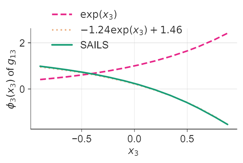
Product-separable interaction, when $R^2_{\text{prod}} \geq \tau$ but $R^2_{\text{lin}} < \tau$. Plot the smoother fitted to the ratios. It recovers the shape of $\phi_l$ up to a scaling that depends on the reference point.

A downward-sloping curve against x3. A dashed exp(x3) reference rises instead, while a dotted rescaled version of it, minus 1.24 times exp(x3) plus 1.46, lies exactly on the solid SAILS curve. — The $x_1 \times x_3$ interaction of the same model. The SAILS curve matches $\exp(x_3)$ only after rescaling, here $-1.24\exp(x_3) + 1.46$.

Read the shape, not the axis values. Recovering $\phi_l$ only up to a factor is not a shortcoming of the estimate: the decomposition $g_{jl} = \phi_j \phi_l$ is itself not unique, since scaling $\phi_j$ by any constant $c$ and $\phi_l$ by $1/c$ leaves $g_{jl}$ unchanged. There is no canonical $\phi_l$ to recover, and the choice of reference point picks one representative out of that family. The product $\phi_j(x_j)\,\phi_l(x_l)$, which is what enters the prediction, is unaffected.

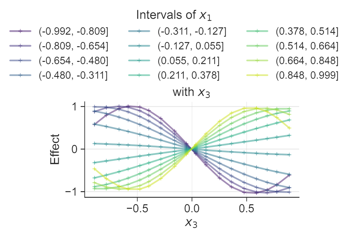
Any interaction. The smooth terms approximate the derivative of the interaction with respect to the FOI, so integrating them over the FOI returns the interaction itself, plus univariate functions of the two features that centering removes. SAILS evaluates the smooth terms on a grid of quantiles of $X_l$, drops grid points outside a term's support so that it never extrapolates, accumulates them across intervals with the trapezoidal rule, and centers the result with respect to both features. This gives one curve of the interaction effect per FOI interval and needs no prior knowledge of the form, so it also covers non-product-separable interactions.

One curve of the interaction effect against x3 per interval of x1, fanning out from zero at x3 = 0 into sine-shaped curves whose amplitude and sign vary with the x1 interval. — The general visualization for a model containing $\sin(\pi x_1 x_3)$, shown interactively at the top of this page. Each curve is one interval of $x_1$.

Each curve shows how the interaction effect varies with $x_l$ at one level of the FOI. Curves are drawn only where their interval has data, which is why they cover a narrower range when the two features are correlated.

Simulation Results

Four settings with nine features $X_1, \ldots, X_9 \sim U(-1,1)$, of which $X_7$ to $X_9$ are noise features. The target is $Y = f(X) + \varepsilon$ with $\varepsilon \sim \mathcal{N}(0, \mathrm{Var}[f]/5)$, over 1000 drawn samples. The results below are for the oracle predictor $\hat f = f$ with $X_1$ as FOI, across 30 repetitions per setting; the paper additionally reports four fitted ML models in its supplementary material.

Setting	Function $f$	Correlation
I	$f_{\mathbf{I}} = 3x_1 + x_2 + \cdots + x_6 + x_1x_2 + x_1\exp(x_3) + x_1^2x_4 + x_1^2\log(\|x_5\|+1) + \sin(\pi x_1x_6)$	$\rho_{jl} = 0$ for all $j \neq l$
II	$f_{\mathbf{II}} = f_{\mathbf{I}}$	$\rho_{12} \approx 0.3$, $\rho_{13} \approx 0.55$, $\rho_{1\{4,7\}} \approx 0.85$, $\rho_{1\{5,6,8,9\}} \approx 0$
III	$f_{\mathbf{III}} = f_{\mathbf{I}} + x_1x_2x_3$	$\rho_{jl} = 0$ for all $j \neq l$
IV	$f_{\mathbf{IV}} = f_{\mathbf{III}} + \cos(\pi x_1x_2x_4) + x_1^2x_5x_6^2$	$\rho_{jl} = 0$ for all $j \neq l$

The four simulation settings: two-way and independent (I), two-way and correlated (II), one linear higher-order term (III), and complex higher-order terms (IV). The figures below show Settings I, II, and IV; the paper reports all four.

Detection Separates Interacting From Noise Features

Boxplots of the approximate p-value per interacting feature in Setting I. The boxes for x2 to x6 sit flat at zero; the boxes for x7 to x9 spread between roughly 0.05 and 0.4, above the dashed 0.05 line. — **(a)** Setting I.

The same boxplot for Setting II with correlated features. The interacting features remain at zero and the noise features, including the strongly correlated x7, stay above the dashed threshold. — **(b)** Setting II.

The same boxplot for Setting IV with complex higher-order interactions. The interacting features stay low, with a slightly raised box for the weaker x5, and the noise features stay mostly above the threshold. — **(c)** Setting IV.

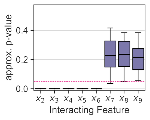
Truly interacting features ($X_2$ to $X_6$) receive values at essentially zero, while the noise features $X_7$ to $X_9$ sit above $\alpha = 0.05$ with few false positives. Correlations do not break this, consistent with ALE's conditional perspective: $X_7$, a noise feature strongly correlated with the FOI, is still correctly called non-interacting. Under complex higher-order interactions the weaker $X_5$ rises somewhat and the false positive rate inflates marginally, which is what surrogate misspecification predicts.

Categorization Is Accurate Under Two-Way Interactions, and Conservative Elsewhere

Boxplots of the linearity measure in Setting I. x2 and x3 sit at 1.0, x4 and x5 at 0.0, and x6 at about 0.35. — **(a)** Setting I: $R^2_{\text{lin}}$.

Boxplots of the linearity measure in Setting II. x2 stays at 1.0 and x3 drops to about 0.93, while x4 rises to about 0.41, x5 stays near 0.0, and x6 sits at about 0.34. — **(b)** Setting II: $R^2_{\text{lin}}$.

Boxplots of the linearity measure in Setting IV. The values for the linear interactions drop below 1.0 but remain clearly above those of the non-linear ones. — **(c)** Setting IV: $R^2_{\text{lin}}$.

Boxplots of the product-separability measure in Setting I. x2 to x5 sit near 1.0 while x6 sits far lower. — **(d)** Setting I: $R^2_{\text{prod}}$.

Boxplots of the product-separability measure in Setting II. x2 and x5 sit at 1.0, x3 drops to about 0.72, x6 sits near 0.13, and the x4 position is empty because the measure could not be computed there. — **(e)** Setting II: $R^2_{\text{prod}}$.

Boxplots of the product-separability measure in Setting IV. All values drop substantially compared with Setting I, including for features not involved in a higher-order term. — **(f)** Setting IV: $R^2_{\text{prod}}$.

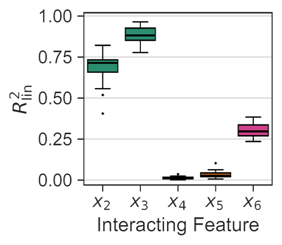
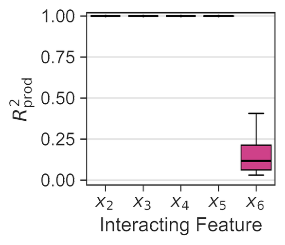
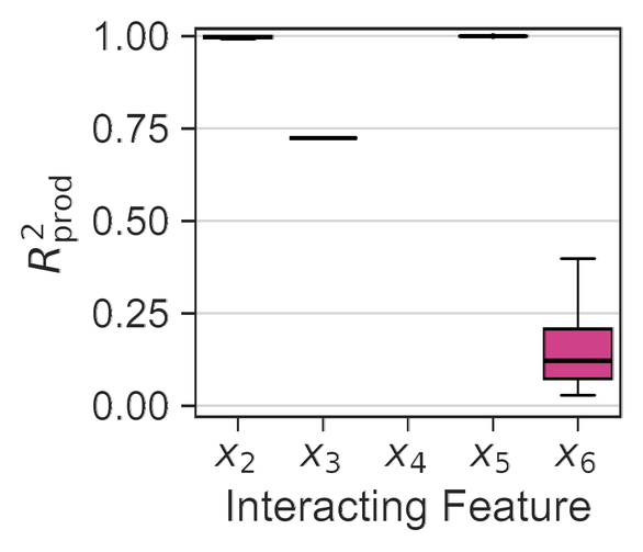
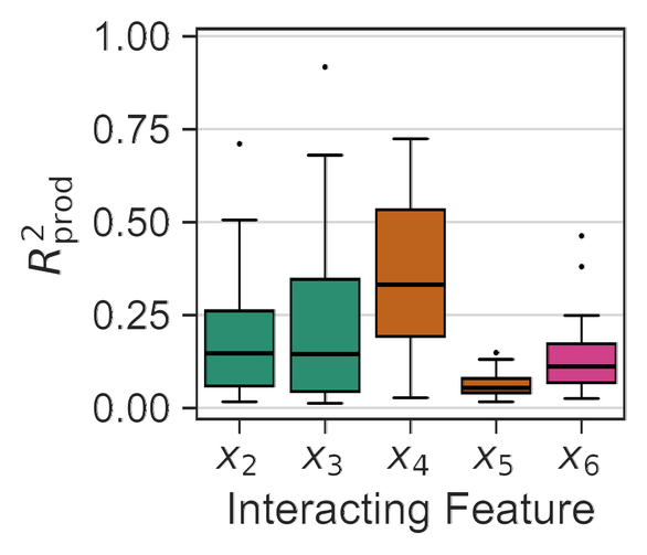
Under two-way interactions and independence, both measures discriminate perfectly: the linear interactions with $X_2$ and $X_3$ reach $R^2_{\text{lin}}$ near one, the product-separable interactions with $X_2$ to $X_5$ reach high $R^2_{\text{prod}}$, and the non-product-separable $X_6$ stays low on both. Under correlations (Setting II), $R^2_{\text{lin}}$ degrades only modestly and still separates linear from non-linear at $\tau = 0.9$, whereas $R^2_{\text{prod}}$ is more sensitive: the correlated $X_3$ falls to roughly 0.72 and is no longer called product-separable, and for the strongly correlated $X_4$ no reference point lies within the support of all smooth terms, so the measure cannot be computed at all. That is the empty position in panel (e).

Higher-order interactions hurt the two measures differently. The non-linear higher-order terms of Setting IV degrade $R^2_{\text{lin}}$, though it stays higher than for genuinely non-linear two-way interactions. $R^2_{\text{prod}}$ breaks down under any higher-order interaction, even for features not involved in one, because misspecified surrogates no longer keep the shapes consistent across intervals. Both measures err on the safe side: they rarely claim linearity or product-separability where there is none.

The General Visualization Recovers Interaction Shapes

Three panels for Setting I showing the recovered interaction effect against x2, x4, and x6, with one curve per interval of x1. The x2 curves are straight lines, the x4 curves are straight lines whose slopes scale non-linearly with the interval, and the x6 curves form sine shapes. — **(a)** Setting I (two-way, independent).

The same three panels for Setting II. The curves for the weakly correlated x2 are largely unchanged, while the curves for the strongly correlated x4 cover a visibly narrower range of the x-axis. — **(b)** Setting II (two-way, correlated).

The same three panels for Setting IV. The curves keep their broad shapes but are less smooth and show additional structure introduced by the higher-order terms. — **(c)** Setting IV (complex higher-order interactions).

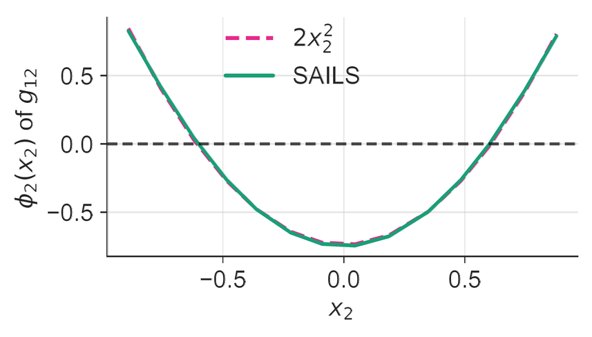
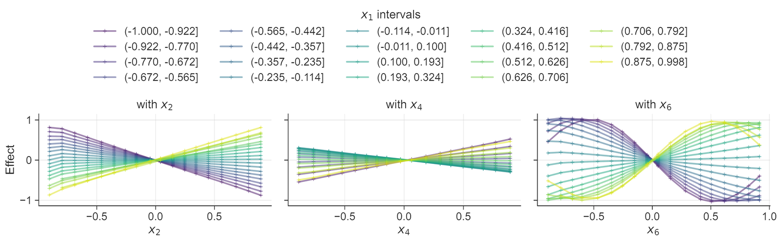
Under independence, the recovered curves match the ground-truth interaction effects closely, and the three interaction types are distinguishable by eye: $X_1 \times X_2$ is linear in both features, $X_1 \times X_4$ gives straight lines that scale quadratically with $X_1$ (product-separable), and $X_1 \times X_6$ reproduces the sine pattern. Correlations barely matter for the weakly correlated $X_2$; for the strongly correlated $X_4$ the interval-specific curves cover less of the feature range, which is deliberate, since SAILS avoids extrapolating, but it also makes the shape harder to pin down. Higher-order interactions introduce artifacts, and the curves become mixtures of the two-way and higher-order effects, which may still carry useful information.

The two form-specific strategies behave as their measures do. Linear visualization is near perfect under independence and loses accuracy under correlations, because of the varying centering. Ratio-based visualization recovers the rescaled true form under independence, apart from trouble at the non-smooth point of $\phi_5$. In Setting IV nothing is categorized as linear or product-separable at all, so neither form-specific plot is produced and the general visualization takes over.

Application: Power Consumption in Tetouan

The Tetouan city power consumption dataset records 52,417 ten-minute observations for the year 2017 in Tetouan, Morocco. Aggregated to hourly values, with the first ten months as training data (85%) and the last two as test data (15%), a tuned XGBoost predicts Zone 1 consumption at $R^2 = 0.94$ on training and $R^2 = 0.92$ on test data. SAILS is then applied to that model with general_diffuse_flows (total solar radiation) as FOI; the surrogates reach an average in-sample $R^2$ of 0.96, so they capture most of the local effect variation (which is a useful measure of faithfulness).

Interacting feature	approx. p-value	Linearity $R^2_{\text{lin}}$	Prod. sep. $R^2_{\text{prod}}$
`Hour`	$1.78 \times 10^{-250}$	0.596	0.271
`Temperature`	$4.37 \times 10^{-119}$	0.191	0.229
`UnixTime`	$1.32 \times 10^{-63}$	0.174	0.111
`diffuse_flows`	$6.19 \times 10^{-32}$	0.023	0.660
`Humidity`	$1.63 \times 10^{-25}$	0.212	0.273
`WindSpeed`	$5.55 \times 10^{-10}$	0.116	0.889

Detection and categorization results. Every feature interacts with the FOI; none clears the categorization threshold $\tau = 0.9$, though WindSpeed comes close to product-separability. The general visualization therefore applies throughout.

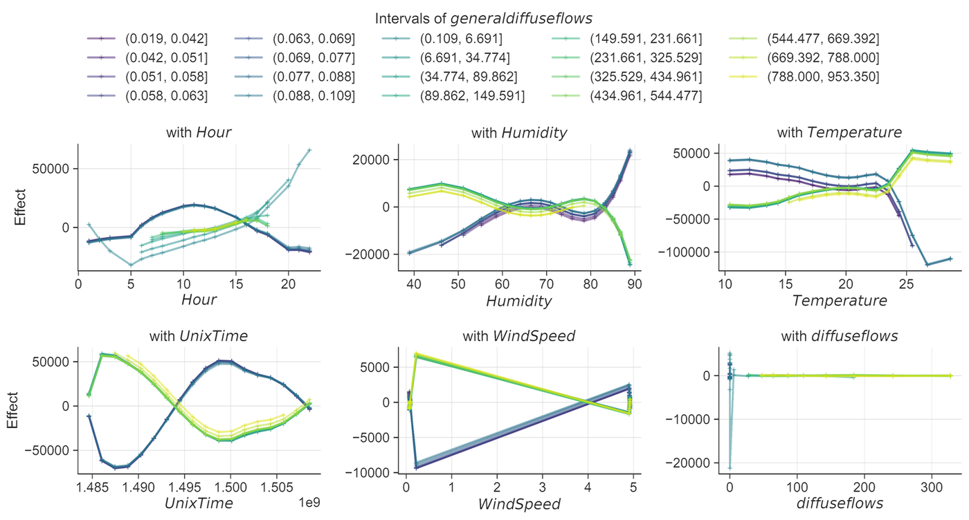
Six panels showing the recovered interaction effect of solar radiation with Hour, Humidity, Temperature, UnixTime, WindSpeed, and diffuse flows. Each panel holds one curve per radiation interval, colored from purple for low to yellow for high radiation. The WindSpeed panel shows near-straight lines of similar shape crossing at one point. — General interaction visualization for `general_diffuse_flows` as FOI. Each curve is one interval of solar radiation, colored from low (purple) to high (yellow).

The recovered patterns line up with plausible demand behavior. For Hour, high radiation has almost no interaction effect, intermediate radiation goes with rising consumption in the evening, and low radiation with higher daytime consumption. Dusk and overcast conditions both call for artificial lighting. High-radiation curves appear only during daytime hours, which shows SAILS respecting the correlation structure instead of extrapolating. Temperature shows a synergistic pattern: low radiation with low temperature raises consumption (lighting plus heating), and so does high radiation with high temperature (cooling). The UnixTime interaction traces the seasons, and the WindSpeed curves indeed share a common shape, consistent with its high product-separability score.

Limitations & Outlook

Regression only. SAILS currently targets regression tasks; extending it to classification through scoring or probability outputs is left for future work.
The central conjecture is unproven. That the smooth terms approximate the FANOVA partial derivatives is supported by classical results for additive models and validated empirically here, but it lacks rigorous guarantees under penalization, finite samples, and fixed basis dimensions.
Categorization is sensitive to correlations. Interval-dependent centering constants shift the smooth terms, which disrupts $R^2_{\text{prod}}$ in particular; for strongly correlated features it may not be computable at all.
Two-way interactions are assumed. The GAM surrogate structure implies at most two-way interactions. Higher-order terms cause misspecification, visible mainly in $R^2_{\text{prod}}$ and in less accurate, less smooth visualizations.

What Comes Next

We plan to turn SAILS into a robust implementation that addresses the open issues above, in particular its sensitivity to correlated features, and to extend it to classification tasks and categorical features. The aim is a model-agnostic, easy-to-use pipeline that works in any tabular setting and comes with interactive visualizations.

Stay tuned!

Cite Us

@article{heiss2026sails,
  title   = {{SAILS}: Surrogate-based Analysis of Interactions via Local Effect Smooths},
  author  = {Hei{\ss}, Timo and Herbinger, Julia and Bischl, Bernd and Casalicchio, Giuseppe},
  journal = {arXiv:2606.09404 [stat.ML]},
  year    = {2026}
}

Setting	Function \(f\)	Correlation
I	\(f_{\mathbf{I}} = 3x_1 + x_2 + \cdots + x_6 + x_1x_2 + x_1\exp(x_3) + x_1^2x_4 + x_1^2\log(\|x_5\|+1) + \sin(\pi x_1x_6)\)	\(\rho_{jl} = 0\) for all \(j \neq l\)
II	\(f_{\mathbf{II}} = f_{\mathbf{I}}\)	\(\rho_{12} \approx 0.3\), \(\rho_{13} \approx 0.55\), \(\rho_{1\{4,7\}} \approx 0.85\), \(\rho_{1\{5,6,8,9\}} \approx 0\)
III	\(f_{\mathbf{III}} = f_{\mathbf{I}} + x_1x_2x_3\)	\(\rho_{jl} = 0\) for all \(j \neq l\)
IV	\(f_{\mathbf{IV}} = f_{\mathbf{III}} + \cos(\pi x_1x_2x_4) + x_1^2x_5x_6^2\)	\(\rho_{jl} = 0\) for all \(j \neq l\)

Interacting feature	approx. p-value	Linearity \(R^2_{\text{lin}}\)	Prod. sep. \(R^2_{\text{prod}}\)
`Hour`	\(1.78 \times 10^{-250}\)	0.596	0.271
`Temperature`	\(4.37 \times 10^{-119}\)	0.191	0.229
`UnixTime`	\(1.32 \times 10^{-63}\)	0.174	0.111
`diffuse_flows`	\(6.19 \times 10^{-32}\)	0.023	0.660
`Humidity`	\(1.63 \times 10^{-25}\)	0.212	0.273
`WindSpeed`	\(5.55 \times 10^{-10}\)	0.116	0.889